 ChipBuddy
← Home
ChipBuddy
← Home
Advanced Timing-Analysis Modes
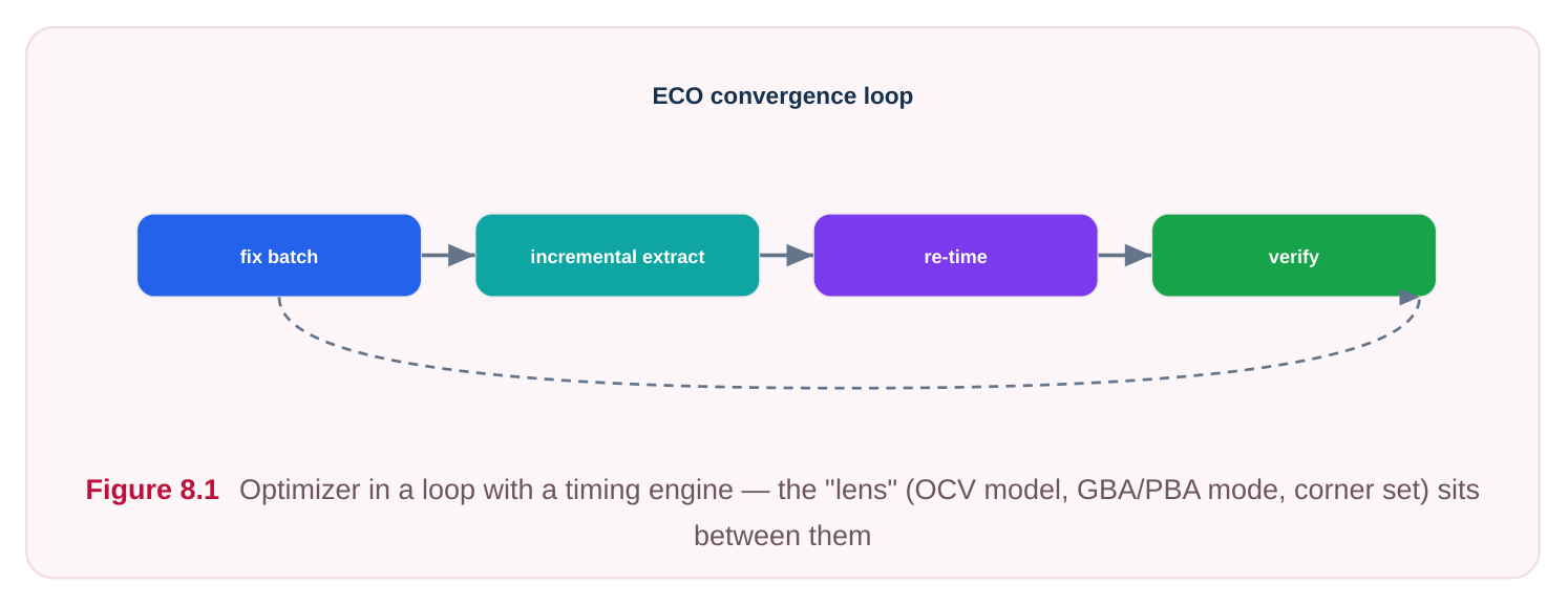
Optimization is only ever as good as the timing picture it is told to fix. An engine that closes a path it never had to touch, or that ignores a violation that signoff later flags, has not done its job well — even if every individual transform it ran was correct. This chapter is about the lens through which the optimizer sees timing: the variation models, the analysis granularity, and the corner-and-mode coverage that together decide whether your work-in-tool effort survives contact with signoff. Get the lens wrong and you either over-fix (burning area, power, and runtime on phantom problems) or underfix (shipping a design that fails the moment a more accurate tool looks at it). The recurring tension in this chapter is accuracy versus runtime. More accurate analysis is slower; faster analysis is more pessimistic or more optimistic. The skill of a physical-design engineer is knowing which knob to turn for which stage of the flow.
Why Optimization Quality Depends on the Analysis Mode
Every optimization transform — buffer insertion, gate sizing, restructuring, useful-skew — is driven by slack. The optimizer asks the timing engine "what is the slack on this endpoint?" and acts on the answer. If that slack number is artificially negative, the optimizer will spend effort, area, and leakage power chasing a violation that does not really exist. If it is artificially positive, the optimizer leaves a real violation untouched. So the analysis mode — how variation is modeled, how a path's delay is computed, which corners and functional modes are considered — is not a passive reporting choice. It is the cost function. Changing the mode changes what the optimizer believes "good" looks like. This is why two flows that run identical transforms can produce designs of very different quality and very different power: they were optimizing against different truths.
On-Chip Variation and Derating
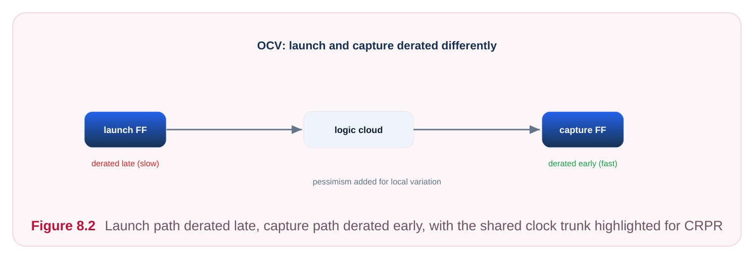
On a real die, two gates sitting micrometers apart do not behave identically. Local variations in transistor channel length, threshold voltage, metal width, temperature, and supply droop mean that the launch path of a flop-to-flop transfer can be running fast while the capture path runs slow — or vice versa. On-chip variation (OCV) is the methodology for modeling this so that a single nominal corner does not paint an unrealistically uniform picture. The classic, simplest form is flat OCV derating: you multiply path delays by a derate factor. For a setup check you want the launch/data path to be slow (so you derate it up, e.g. ×1.05) and the capture/clock path to be fast (derate down, e.g. ×0.95). For a hold check you reverse the sense. This pushes launch and capture apart and forces the optimizer to leave margin for the case where local conditions conspire against you.
# illustrative — generic, not tool-specific
# Setup: make data paths slow, clock-capture paths fast
set_timing_derate -late  1.05 -data       ;# launch/data slower
set_timing_derate -early 0.95 -clock       ;# capture clock faster
# Hold uses the opposite early/late assignment
The problem with flat derating is that it is blunt. A constant multiplier ignores the fact that variation does not scale linearly with path depth, and that nearby cells are correlated. Advanced/parametric OCV (often AOCV, or a distance/depth-dependent derate) addresses this: derate factors become a function of how many stages a path has and how physically spread out it is. A long, deep path sees a smaller per-stage derate because random local variations partially cancel along the way (statistical averaging), while a short path keeps a larger derate. The result is less pessimism on exactly the deep paths that flat OCV punishes hardest.
| OCV concept | What it models | Effect on the optimizer |
|---|---|---|
| Flat OCV derate | Constant multiplier on path delay | Simple, uniformly conservative; |
over-margins deep paths
| Depth/stage-aware derate | Derate shrinks with path depth | Recovers pessimism on deep paths; |
|---|---|---|
| (AOCV-style) | (averaging) | fewer needless fixes |
| Distance-aware derate | Larger derate for physically spread-out paths | Captures spatial correlation more faithfully |
| Clock reconvergence pessimism | Common clock segment shared | Cancels double-counted derate on |
| removal (CRPR) | by launch & capture | the shared clock path |
A critical companion to OCV is clock reconvergence pessimism removal (CRPR). When launch and capture clocks share a common path up to a divergence point, naive OCV derates that common segment as both early and late simultaneously — which is physically impossible. CRPR credits back that double-counted pessimism. Without it, the optimizer over-fixes paths whose clocks share a long common trunk. The whole OCV machinery is a form of graph-based pessimism: derates are applied per-arc on the timing graph, conservatively, regardless of which specific combination of arcs a real path actually uses. That conservatism is the price of speed — and it sets up the next distinction.
Graph-Based vs Path-Based Analysis
Graph-based analysis (GBA) propagates a single worst-case arrival and a single worst slew through each node of the timing graph. At every node it keeps the worst incoming value and pushes it forward.
This is fast — it is essentially one sweep of the graph — and it is what optimization engines lean on for most of their inner-loop slack queries. But it is pessimistic: the worst slew arriving at a node may come from input A, while the worst arrival propagating onward goes to output B; GBA combines them even though no single real path ever experiences both simultaneously. It also tends to apply the worst perarc derate everywhere. Path-based analysis (PBA) takes a specific path end to end and recomputes its delay using the actual slews propagating along that path, and the derates appropriate to that path's depth. Because it stops mixing worst-cases from different paths, PBA almost always reports better (less negative) slack than GBA. The difference — the recovered pessimism — can be hundreds of picoseconds on slewsensitive or deep paths.
| Aspect | Graph-Based Analysis (GBA) | Path-Based Analysis (PBA) |
|---|---|---|
| Granularity | Per-node worst values | Per-path recomputation |
| Slew handling | Worst slew at each node, mixed | Actual slew along the chosen path |
| Pessimism | High (safe but over-conservative) | Recovered toward reality |
| Runtime | Fast — single graph sweep | Slow — re-traces each path |
| Typical use | Inner-loop optimization, early triage | Final timing recovery, signoff cleanup |
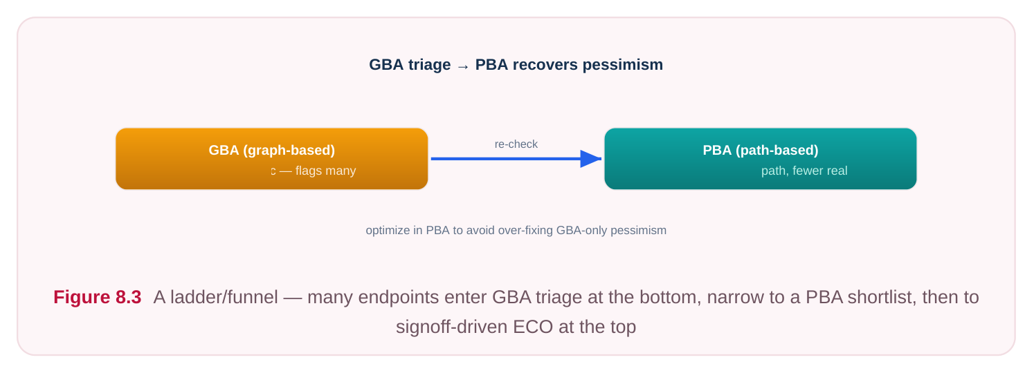
The optimization implication is large. If you optimize purely against GBA, you will over-fix: the engine will keep upsizing and buffering paths that PBA would have shown as already passing. That wastes area and burns leakage power. The mature flow uses PBA-aware optimization — the engine queries the path-based slack before committing a transform, so it only acts on paths that are genuinely failing once pessimism is removed.
# illustrative — generic, not tool-specific
# Recompute critical paths path-based to recover GBA pessimism
set_analysis_mode -path_based true -effort high
# Let optimization consult PBA slack before fixing
optimize_timing -mode path_based -avoid_overfix
report_timing -path_based -nworst 20
A practical pattern: run GBA to quickly find the candidate violating endpoints (cheap), then run PBA only on that shortlist to decide which actually need work (accurate). You pay PBA's runtime only where it matters, and you avoid both blanket over-fixing and the cost of running PBA on the whole design.
Multi-Corner Multi-Mode Signoff-Driven Optimization
A modern SoC must work across many corners (process / voltage / temperature combinations plus RC extraction variants) and many functional modes (functional, test/scan, sleep, low-power). A path that has slack to spare in one mode-corner can be the critical path in another. Optimizing against a single corner is a recipe for fixing one scenario while breaking another.
Multi-corner multi-mode (MCMM) analysis evaluates every relevant scenario together and lets the optimizer reason about the worst across all of them per endpoint. The classic split: setup tends to be limited by slow/low-voltage/high-temp corners, while hold tends to be limited by fast/high-voltage/lowtemp corners — so you must hold both in view simultaneously, because a hold fix in the fast corner (adding delay) must not create a setup failure in the slow corner.
| Scenario role | Typically limiting for | Why |
|---|---|---|
| Slow process, low V, hot | Setup | Maximum cell delay |
| Fast process, high V, cold | Hold | Minimum cell delay |
| Functional mode | Mission-mode setup/hold | Real operating clocks |
| Test/scan mode | Shift/capture timing | Higher or gated clock activity |
| Low-power / retention mode | Setup at reduced voltage | Slower transistors at low V |
The deeper issue is agreement with signoff. The in-tool timing engine inside an implementation flow is usually faster and slightly less accurate than the dedicated signoff timing tool. If the optimizer closes timing against its own internal numbers but signoff disagrees, you get a frustrating loop of "clean in the tool, failing at signoff." Signoff-driven optimization breaks that loop: the implementation engine hands violating paths to the signoff-grade analysis, gets back authoritative slack, and only then generates fixing ECOs. Because in-tool and signoff now share one source of truth, the ECO that closes timing in analysis also closes it in the implementation database.
# illustrative — generic, not tool-specific
# Define the MCMM scenario set, then optimize against signoff slack
create_scenario -name func_slow_setup -mode func -corner slow_lowv_hot
create_scenario -name func_fast_hold  -mode func -corner fast_highv_cold
set_active_scenarios {func_slow_setup func_fast_hold scan_slow_setup}
# Hand paths to signoff engine, fetch authoritative slack, emit ECO
signoff_optimize -scenarios [get_active_scenarios] \
-fix {setup hold} -mode path_based \
-output eco_fixes.tcl
The discipline here is to keep the constraints identical between implementation and signoff — same clock definitions, same exceptions, same derates — so the two engines never diverge for reasons unrelated to engine accuracy.
Rule-File Driven Optimization and Case Analysis
Two further inputs quietly shape what the optimizer is allowed to see and do. Rule-file / constraint-file driven optimization means the engine respects an external set of design rules and exceptions during fixing: max transition, max capacitance, max fanout, plus timing exceptions like false paths and multicycle paths. These exceptions matter enormously for optimization
quality. A path marked false should be invisible to the optimizer — if the exception is missing, the engine wastes effort closing a path that can never propagate a real transition. A multicycle path should be timed against its true number of cycles, not one — otherwise the optimizer over-constrains it and adds needless buffers.
# standard (SDC)
set_false_path   -from [get_pins cfg_reg/CK]            ;# never time this
set_multicycle_path 2 -setup -from [get_pins mac/*]     ;# 2-cycle path
set_max_transition 0.150 [current_design]               ;# rule the opt must honor
set_max_capacitance 0.080 [get_ports data_out*]         ;# rule the opt must honor
Case analysis sets constant values on certain pins (e.g. tying a test-enable to 0, or a mode-select to a fixed value) so the engine only analyzes — and only optimizes — the logic that is actually active in that configuration. This both prunes impossible paths (improving accuracy and runtime) and prevents the optimizer from fixing logic that is disabled in the mode under analysis.
# standard (SDC)
set_case_analysis 0 [get_ports test_enable]   ;# functional mode: scan off
set_case_analysis 1 [get_ports mode_select]    ;# pick the active configuration
The catch: case analysis is per scenario. In MCMM, the scan mode wants test_enable = 1 , the functional mode wants test_enable = 0 . If you accidentally apply one mode's case analysis globally, the optimizer optimizes the wrong logic. Correct MCMM setup binds each set_case_analysis to the scenario it belongs to, so each mode sees its own legitimate paths.
The Accuracy-vs-Runtime Trade-off Across Modes
Putting the pieces together, the modes form a ladder from fast-and-rough to slow-and-authoritative. A well-run flow climbs this ladder: cheap modes early to make big structural moves, expensive modes late to converge on signoff truth.
| Analysis mode | Accuracy | Runtime | When to use |
|---|---|---|---|
| Single corner, flat OCV, GBA | Low | Fastest | Early placement/synthesis, coarse |
structural opt
Single corner, AOCV-style, GBA + Medium Fast Mid-flow opt; pessimism partly recovered
MCMM, AOCV-style, GBA + CRPR Medium- Moderate Multi-scenario optimization through route
MCMM, AOCV-style, PBA on critical High Slow Late timing recovery, avoiding over-fix
MCMM, signoff engine, PBA, full Highest Slowest Final signoff-driven ECO closure
The headline rule: never optimize in a mode more pessimistic than the one you will sign off in. Doing so guarantees wasted area and power on paths that the signoff lens would have passed. Equally, never sign off in a mode more accurate than the one you optimized in without a final convergence pass — that is how "clean in tool, broken at signoff" happens.
Interview Q&A
keeps a single worst arrival and worst slew at each node and propagates them forward, even though the worst slew and the worst onward arrival may come from different incoming paths. It effectively combines worst-cases that no single real path experiences, and applies worst-case per-arc derates everywhere. PBA re-traces an actual path end to end with the real slews and depth-appropriate derates along that path, so it stops mixing unrelated worst-cases. The recovered slack means the optimizer fixes fewer paths — only those genuinely failing under realistic conditions.
removal credits back the derate that OCV double-counts on the clock segment shared by both the launch and capture clocks. That common trunk cannot be simultaneously early and late, yet OCV treats it as both. Without CRPR, paths whose launch and capture clocks share a long common path look artificially worse, and the optimizer wastes effort and area fixing them. CRPR is essential to avoid systematic over-fixing on designs with deep shared clock trees.
engine? The implementation engine is fast but slightly less accurate than the dedicated signoff timing tool, so closing timing against in-tool numbers can still leave signoff failing. Signoff-driven optimization sends violating paths to the signoff-grade analysis, gets authoritative slack back, and generates ECOs against that. Because both share one source of truth — and identical constraints — an ECO that closes timing in analysis also closes it in the implementation database, eliminating the "clean in tool, failing at signoff" loop.
you avoid it? Setup is typically limited by the slow corner (max delay) while hold is limited by the fast corner (min delay). Fixing hold means adding delay — usually in the fast corner — but that same added delay increases path delay in the slow corner, eating setup margin. You avoid it by optimizing
with all relevant scenarios active simultaneously, so the engine sees the worst setup and worst hold per endpoint at once and only inserts delay where it does not break setup anywhere. Per-scenario case analysis and consistent constraints keep each mode honest.
Key Takeaways
- The analysis mode is the optimizer's cost function: change the lens and you change what "optimized" means. Wrong lens means over-fixing (wasted area/power) or under-fixing (signoff failures).
- OCV models that launch and capture paths see different local conditions; derates push them apart, AOCV-style depth/distance awareness recovers pessimism on deep paths, and CRPR cancels double-counted pessimism on shared clock trunks.
- GBA is fast but pessimistic because it mixes per-node worst-cases; PBA re-traces real paths to recover slack. Use GBA to triage, PBA to decide, to avoid over-fixing.
- MCMM holds all corners and modes in view together so setup fixes do not break hold and vice versa; signoff-driven optimization makes in-tool and signoff agree by sharing one authoritative slack source.
- Honor exceptions (false/multicycle paths), design rules (max transition/cap/fanout), and per- scenario case analysis so the optimizer only ever works on legitimately active, legitimately failing logic.
- Climb the accuracy ladder: cheap modes for early structural moves, expensive signoff-grade PBA for final closure — and never optimize in a mode more pessimistic than the one you sign off in.
Comments
Leave a Reply