 ChipBuddy
← Home
ChipBuddy
← Home
Quick Reference & Appendix
14.1 Essential Commands Checklist
Before you walk into a CTS interview, you should be able to recite the core command set from memory and explain what each one actually does to the design database. This subsection is your cheat sheet. Think of it less as a tutorial and more as the laminated card you keep next to the key‐ board. Clock tree synthesis is a sequenced activity: you describe the clocks, you settle the placement, you bound the electrical behavior, you sanity-check the tree topology, you tune the engine, you build, and finally you measure. The commands below map onto that rhythm. The exact spelling varies a little between tool vendors, but the intent transfers cleanly across any flow.
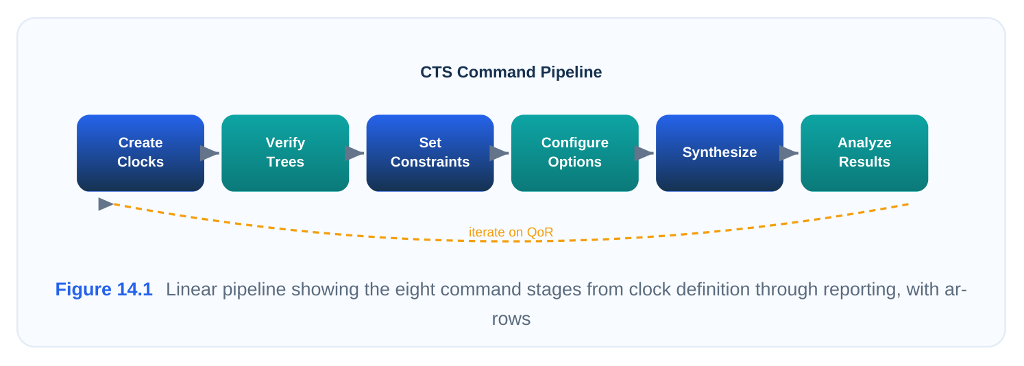
Defining and Deriving Clocks
Everything starts with telling the tool what a clock is. A primary clock is anchored to a real port or pin and given a period; a generated (or derived) clock is computed from another clock through a divider, multiplier, or gating cell.
# Primary clock: 800 MHz reference arriving at the clk_in port
create_clock -name SYS_CLK -period 1.2 [get_ports clk_in]
# Generated clock: a divide-by-2 produced by a flop's Q output
create_generated_clock -name DIV2_CLK \
-source [get_ports clk_in] \
-divide_by 2 \
[get_pins div_reg/Q]
If you forget the generated clock, the tool treats the divider output as ordinary logic and never balances it as part of the tree — a classic cause of mysterious downstream skew. Always verify that every flip-flop clock pin is reachable from a defined clock object.
Settling Placement Before Building
CTS assumes a stable placement. The locations of the sinks are the coordinates the tool routes to, so you commit placement first.
place_design
check_legality -verbose
check_legality -verbose  is non-negotiable. Overlapping or off-grid cells will sabotage buffer
insertion later, and the -verbose switch tells you which instances are illegal instead of just reporting a count.
Bounding Electrical Behavior
You then cap the two electrical quantities that drive buffer sizing: the load each driver sees and how fast each net transitions.
set_max_capacitance 0.55 [current_design]
set_max_transition  0.18 [get_clocks *]
Topology Check, Engine Setup, Build, and Report
| Command | Stage | What it does |
|---|---|---|
| check_clock_trees | Pre-build audit | Flags undefined sinks, ignored pins, exceptions, and structural problems before you spend runtime |
| set_c‐ | Engine lock_tree_options | Sets target skew, effort, buffer/inverter lists, routing layers setup |
| synthes‐ | Build | Inserts and balances the buffer network |
ize_clock_trees
report_clock_tree	Measure	Structural summary: depth, buffer count, fanout
report_clock_timing	Measure	Skew, latency, and insertion delay per clock
A clean check_clock_trees run before synthesis saves you from discovering structural surprises only after a long build.
14.2 Design Rule Defaults and Ranges
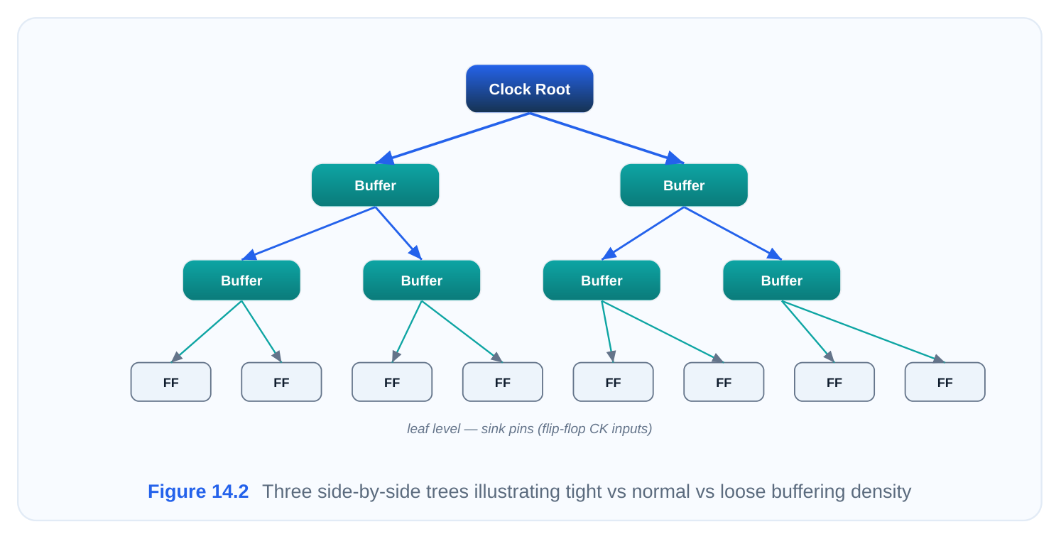
Constraints are the lever you pull most often, so internalize sensible starting values. Two of them — maximum capacitance and maximum transition — directly govern how aggressively the tool buffers the tree. Tighten them and you get more, smaller buffers (better signal integrity, more area and power). Loosen them and you save resources at the cost of slope and robustness. Below are widely used reference bands. Treat "normal" as your default and reach for "tight" or "loose" only when timing, power, or area pressure justifies it.
| Constraint | Tight | Normal | Loose | Unit | What tightening buys you |
|---|---|---|---|---|---|
| Max capacitance | 0.35 | 0.55 | 0.95 | pF | Cleaner edges, lower delay sensitivity, more buffers |
| Max transition | 0.13 | 0.18 | 0.45 | ns | Sharper slopes, better hold robustness, more power |
| Target skew | ~45 | ~90 | ~135 | ps | Tighter balancing, more insertion delay/area |
How to Read the Bands
The numbers are technology-relative — a 5 nm node will use far smaller absolute caps than these illustrative values — but the relationships hold everywhere. A tighter max-transition forces the tool to keep slopes crisp, which improves on-chip-variation (OCV) behavior and hold timing because slow edges amplify uncertainty. A tighter max-cap limits how many sinks a single buffer is allowed to drive, increasing the tree's branching.
Target skew deserves a word of caution: "auto" or tool-derived skew targets in the 45–135 ps range are fine for most blocks, but driving skew to near zero is rarely free. The buffers added to perfectly balance arrival times consume area, burn dynamic power, and can themselves introduce variation. A small, deliberate skew budget is healthier than a heroic zero-skew chase.
14.3 Decision Framework
When a CTS result misses a goal, you do not randomly twist knobs — you diagnose the dominant fail‐ ure mode and apply the recipe matched to it. The framework below is the single most interview-friendly mental model in this chapter. Memorize the four branches.
| Symptom | Root cause focus | Recommended actions |
|---|---|---|
| Timing fail‐ | Skew and latency too large ing | high_effort mode, target_skew 0.045 , max_transition 0.135 |
| Power too | Excess switching/leakage in | Enable dynamic + leakage power optimization; prefer low- |
| high | clock net | power buffers |
| DRC viola‐ | Routing/placement legality tions | Advanced legalization, restrict/add routing layers, fix place‐ ment |
| Area too | Too many CTS buffers large | power_reduction , skew_only balancing, loosen max- cap/transition |
Working the Branches
If timing is failing, you want the engine to spend more effort balancing and to keep edges fast. Push effort up, tighten the skew target so arrival times converge, and tighten transition so slopes stay sharp (slow slopes inflate setup and hold uncertainty under OCV).
set_clock_tree_options -effort high
set_clock_tree_options -target_skew 0.045
set_max_transition 0.135 [get_clocks *]
synthesize_clock_trees
If power is the problem, the clock network is almost always the biggest single dynamic-power con‐ sumer on the die because it switches every cycle. Turn on dynamic and leakage optimization and bias the buffer library toward low-power, higher-Vt cells. If DRC is the issue, the tree is electrically fine but physically illegal — buffers landing on blockages, routes on congested layers. Escalate legalization, steer clock routes onto cleaner metal layers, and revisit placement density in the offending region. If area is the concern, you are paying too much silicon for balancing precision you may not need. Switch to a skew-reduction-only objective, enable power/area reduction, and relax the electrical caps so fewer buffers are required.
14.4 Option Interaction Matrix
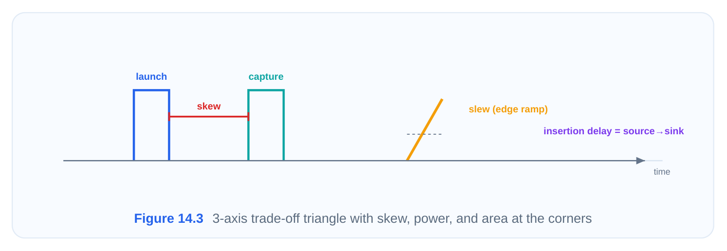
Options do not act in isolation. Some reinforce each other; some quietly cancel each other out. The matrix below captures the combinations interviewers love to probe. The principle to articulate: every CTS option trades among the three currencies of skew, power, and area, and you can only push two at once.
Interac‐
Option A Option B Why
| High effort | Tight target | Syner‐ | More effort lets the engine actually hit an aggressive skew |
|---|---|---|---|
| skew | gistic | goal | |
| Tight max- | Low-power | Conflict‐ | Sharp slopes need stronger drivers; low-power cells fight |
| transition | buffers | ing | that |
| Skew-only bal‐ | Power reduc‐ ancing | Syner‐ tion | Both reduce buffer count and resource use gistic |
| Tight max-cap | Area reduction | Conflict‐ | Lower cap forces more buffers, enlarging area |
ing
| Useful skew | Tight target | Conflict‐ | Useful skew deliberately introduces skew; a tight global tar‐ |
|---|---|---|---|
| skew | ing | get erases that freedom | |
| Multi-layer rout‐ | DRC-clean ing | Syner‐ goal | More layer choices relieve congestion and DRC pressure gistic |
Reading the Matrix in an Interview
The two synergistic pairs to remember are (high effort + tight skew) and (skew-only + power reduc‐ tion). The two conflicts that trip people up are (tight transition vs low-power cells) and (useful skew vs tight global skew). That last one is subtle and worth rehearsing aloud: useful skew is a technique where you intentionally delay or advance certain clock arrivals to borrow time across tight paths. If you simultaneously command the tool to drive global skew toward zero, you have told it to both create and destroy skew. The two objectives are mutually defeating, and the tool will give you a muddled compromise. Pick one strategy per region.
14.5 Pre-CTS Command Flow
This is the canonical ordered sequence. If an interviewer asks "walk me through your CTS flow," recite these ten steps in order. The ordering is not arbitrary — each step depends on the state established by the one before it.
# 1. Define all primary and generated clocks
create_clock -name SYS_CLK -period 1.2 [get_ports clk_in]
create_generated_clock -name DIV2_CLK -source [get_ports clk_in] \
-divide_by 2 [get_pins div_reg/Q]
# 2. Apply timing constraints / read the SDC
set_clock_uncertainty 0.05 [get_clocks *]
set_clock_latency -source 0.3 [get_clocks SYS_CLK]
# 3. Complete and legalize placement
place_design
check_legality -verbose
# 4. Set electrical design rules
set_max_capacitance 0.55 [current_design]
set_max_transition  0.18 [get_clocks *]
# 5. Configure the CTS engine
set_clock_tree_options -effort high -target_skew 0.09 \
-buffer_list {CKBUFX4 CKBUFX8} -inverter_list {CKINVX4}
# 6. Pre-build structural audit
check_clock_trees
# 7. Build the clock tree
synthesize_clock_trees
# 8. Report structure
report_clock_tree
# 9. Report timing
report_clock_timing
# 10. Post-CTS optimization (fix residual setup/hold, hold-buffer insertion)
optimize_clock_tree
The Logic of the Ordering
| Step | Depends on | If skipped |
|---|---|---|
| 1 Clocks | Nothing | Sinks go unbalanced; generated clocks ignored |
| 2 Constraints | Step 1 | Uncertainty/latency unmodeled; optimistic timing |
| 3 Placement | Step 2 | No fixed sink coordinates to route to |
| 4 DRCs | Step 3 | Buffers sized blindly; SI risk |
| 5 Engine opts | Step 4 | Default effort/skew; suboptimal tree |
| 6 Audit | Step 5 | Structural surprises after long build |
| 7 Build | Step 6 | — |
| 8–9 Reports | Step 7 | No visibility into quality |
| 10 Post-opt | Steps 7–9 | Residual hold/setup violations remain |
The most common ordering mistake is running CTS before placement is legal, or before generated clocks exist. Both produce trees that look built but are silently wrong.
14.6 Example Scenarios
Abstract rules stick better when attached to concrete designs. Here are four archetypes you will encounter, each with a recommended option recipe. In an interview, naming the dominant constraint first and then justifying the recipe is exactly the reasoning structure evaluators want to see.
Scenario 1 — Timing-Critical Processor Core
The dominant pressure is performance. The clock period is tight, paths are dense, and every picosecond of skew eats directly into the timing budget.
set_clock_tree_options -effort high -target_skew 0.045
set_max_transition 0.135 [get_clocks *]
set_max_capacitance 0.35 [current_design]
synthesize_clock_trees
optimize_clock_tree
Rationale: maximum effort plus an aggressive skew target gives the balancer room to converge; tight transition and cap keep edges crisp so OCV does not erode the margin you fought for. You accept the extra buffers and power as the price of frequency.
Scenario 2 — Low-Power IoT Chip
Here the clock runs slowly and battery life is everything. The clock network is the top dynamic-power offender, so the recipe inverts the processor recipe.
| Setting | Value | Reason |
|---|---|---|
| Effort | medium | Skew budget is generous; no need to over-invest |
| Target skew | 0.135 | Loose target = fewer balancing buffers |
| Buffer library | low-power / high-Vt | Minimize leakage and switching power |
| Power opt | dynamic + leakage on | Clock net dominates active power |
| Clock gating | aggressive | Stop the clock where it isn't needed |
Scenario 3 — High-Congestion SoC
The design is routable in principle but physically crowded. Timing and power are secondary to simply getting a legal, DRC-clean tree.
set_clock_tree_options -effort medium -target_skew 0.09 \
-routing_layers {M4 M5 M6}
set_clock_tree_options -legalization advanced
synthesize_clock_trees
Rationale: give the router more (and cleaner) layers, escalate legalization, and keep the skew target relaxed so the tool spends its effort on placement legality rather than picosecond balancing it cannot physically achieve.
Scenario 4 — Multi-Domain System
Several asynchronous or ratio-related clock domains coexist. The danger is balancing domains against each other when they should be independent, and mishandling the crossings.
| Concern | Action |
|---|---|
| Domain independence | Balance each clock tree separately; do not force a common skew |
| Clock crossings | Treat CDC paths with proper exceptions; do not balance across them |
| Shared resources | Watch contention for routing layers between domains |
| Generated clocks | Confirm each derived clock is defined and balanced within its own domain |
The interview key phrase: balance within a domain, decouple across domains.
14.7 Sign-Off Checklist
CTS is "done" only when it passes a four-part review covering tree quality, physical legality, power/ area budgets, and completeness. Use this as the literal checklist you walk before declaring victory. Anything unchecked is a reason to iterate.
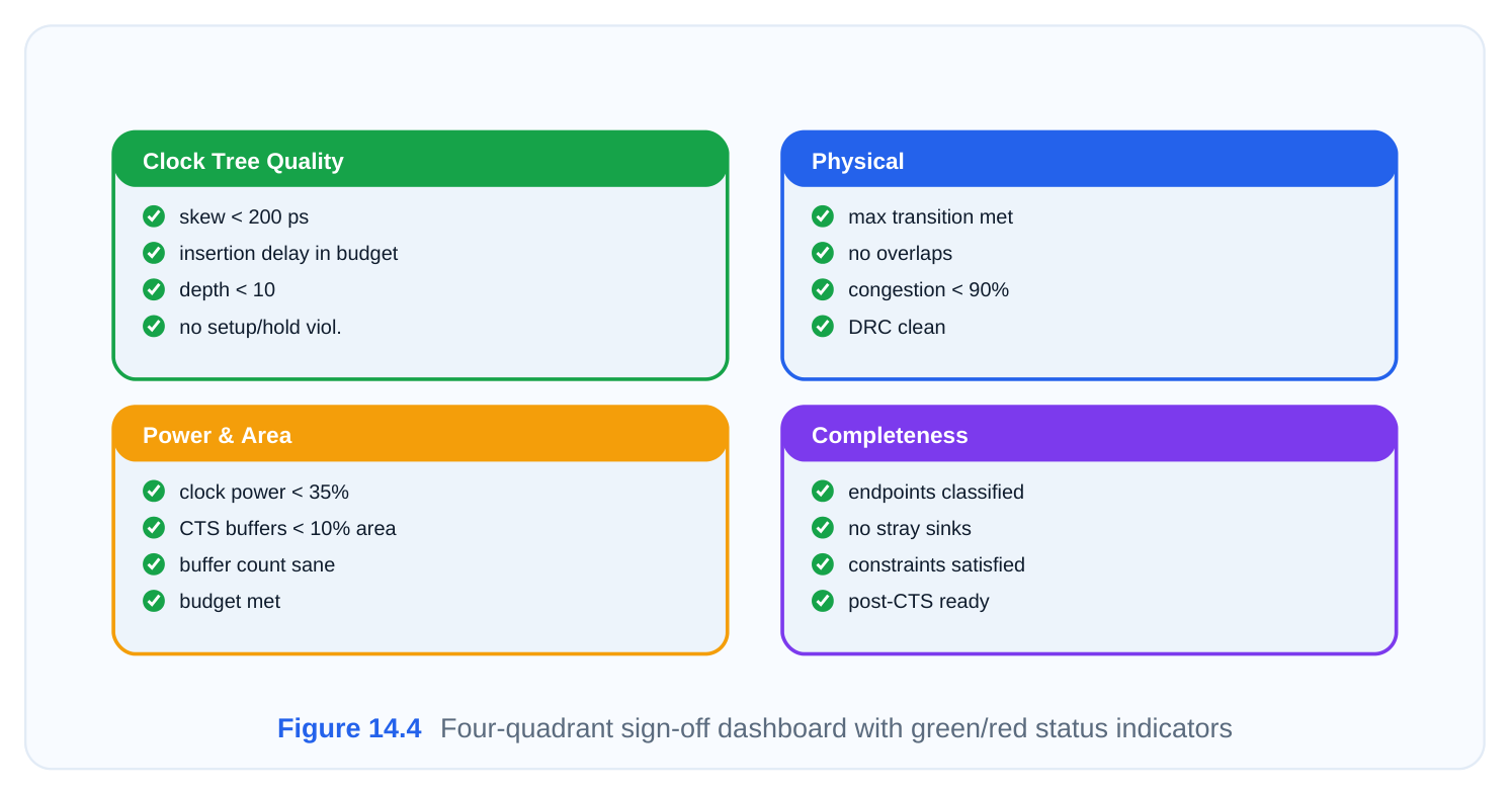
Clock Tree Quality
- [ ] Global skew below 180 ps (or within the block's stated budget)
- [ ] Insertion delay (source latency) inside the planned budget — not drifting high
- [ ] Tree depth under ~12 buffer levels (deeper trees accumulate variation)
- [ ] No setup violations on clock-bounded paths
- [ ] No hold violations after hold-buffer insertion
Physical Quality
- [ ] Maximum transition constraint met on every clock net
- [ ] No overlapping or out-of-bounds CTS buffers
- [ ] Local congestion below ~88% in clock-routing regions
- [ ] DRC clean for clock nets (spacing, via, antenna)
Power and Area
| Metric | Target | Why it matters |
|---|---|---|
| Clock power share | < 33% of total | Clock switches every cycle; the biggest single power lever |
| CTS buffer area | < 9% of block area | Over-buffering signals an unbalanced cost/benefit |
| Buffer count | "reasonable" for sink count | A sudden spike flags a too-tight skew target |
Completeness
- [ ] All endpoints correctly classified (sink vs ignore vs stop pin)
- [ ] No unintended sinks pulled into the tree (stray latches, test logic)
- [ ] All clock constraints satisfied (no dropped or conflicting exceptions)
- [ ] Database is post-CTS ready — propagated clocks enabled for downstream routing and timing closure A passing checklist means propagated-clock timing (not ideal-clock) now governs the design, and you can hand off to detailed routing with confidence.
Interview Q&A
create_clock defines a primary clock anchored to a real port or pin with an explicit period. cre‐ate_generated_clock derives a clock from an existing one through a division, multiplication, or gating relationship — for example a divide-by-2 flop output. Forgetting the generated clock means the tool treats that net as ordinary logic and never balances it.
of the sinks. If cells are overlapping or off-grid, those coordinates are invalid, buffer insertion goes wrong, and you discover the damage only after a long build. check_legality -verbose confirms a clean starting point.
(around 0.05), and tighten max-transition (around 0.13 ns) so edges stay sharp and OCV does not erode margin. Then rerun synthesis and post-CTS optimization.
toggles on every cycle across the entire design, unlike data logic that switches only when activity demands. That makes clock gating, low-power buffers, and a relaxed skew budget the highestleverage power savings.
erately introduces arrival-time differences to borrow time across critical paths. A near-zero global target
instructs the tool to eliminate exactly those differences. The two objectives cancel, producing a muddled compromise. Choose one strategy per region.
Key Takeaways
- Follow the sequence. Define clocks (including generated ones), constrain, legalize placement, set DRCs, configure the engine, audit, build, report, then post-optimize — in that order.
- Know your bands. Normal defaults are roughly 0.55 pF max-cap, 0.18 ns max-transition, and a ~90 ps skew target; tighten or loosen only when a specific pressure justifies it.
- Diagnose before you tune. Match the dominant symptom — timing, power, DRC, or area — to its recipe rather than twisting knobs at random.
- Respect the trade-off triangle. Skew, power, and area pull against each other; you can optimize two at the expense of the third.
- Sign off rigorously. Tree quality, physical legality, power/area budgets, and completeness all have to pass before the design is propagated-clock ready for routing.
Comments
Leave a Reply