 ChipBuddy
← Home
ChipBuddy
← Home
Power-Switch Prototyping & Planning
Every chapter up to now has treated the power-gated domain as something you draw a boundary around and then shut off. This chapter is about the machinery that actually does the shutting off: the power-switch network — the fabric of header or footer transistors that sits between the always-on supply and the switchable rail of a power domain. The central message is that this fabric is expensive enough, and unforgiving enough, that you must prototype and plan it before you commit to a full implementation. Get it wrong and you will either waste silicon on thousands of switches you did not need, or you will build a domain that droops, rings up slowly, and trips your acknowledge logic. Planning sits squarely between floorplanning (where the voltage areas were carved out) and powergrid construction (where the always-on straps were drawn). This is the deepest, most quantitative chapter in the handbook, because switch planning is where physical intuition, current math, and timing all collide.
9.1 Why the Switch Fabric Deserves Its Own Planning Stage
When a domain is on, the switch network is in series with everything it powers. That has three consequences that drive the whole discipline:
- 1. It costs area. Switches are real transistors with real footprints. A large domain can need hundreds
or thousands of them, and they consume routing tracks and placement sites that logic could otherwise use.
- 2. It costs always-on routing. The switch enable signal, and any acknowledge return, must be
routed on the always-on supply and reach every switch. This is overhead that exists purely to control power, not to do computation.
- 3. It costs voltage. A switch in its on-state is a resistor. Every milliohm of effective on-resistance turns
into IR drop on the switched rail, eating into the timing margin of the very logic you are trying to power.
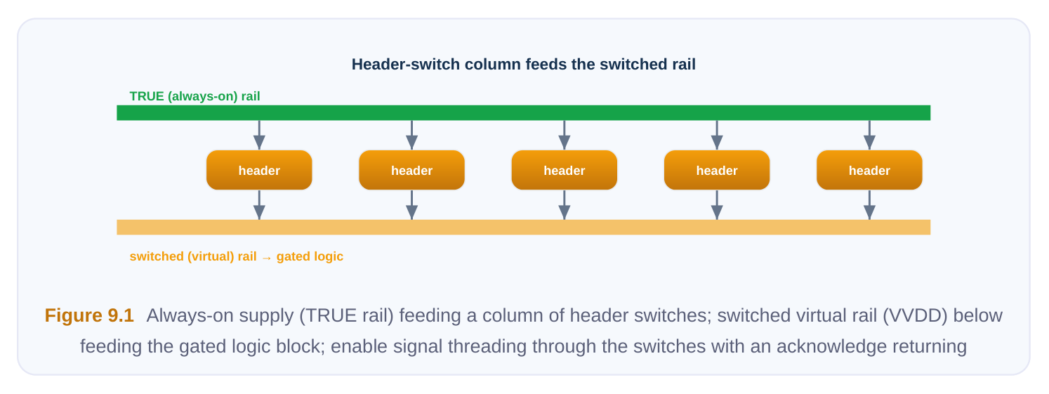
So the planner's job is a balancing act. More switches lower on-resistance and IR drop, but cost area, leakage, and a longer enable chain. Fewer switches save all of that, but risk voltage droop under load and a dangerously fast, current-spiking ramp when the domain wakes up. You cannot find the sweet spot by guessing — you prototype, measure, and iterate.
| Switch concern | Symptom if under-provisioned | Symptom if over-provisioned |
|---|---|---|
| On-resistance / IR | Switched rail sags; timing fails in on-state | Wasted; diminishing returns past a point |
drop
Inrush / ramp current Huge current spike collapses the always- Ramp unnecessarily slow
| Area | — | Domain bloats; placement congestion |
|---|---|---|
| Leakage in off-state | — | Higher residual leakage defeats power |
gating
Enable-chain length Acknowledge arrives too early (false Wake-up latency too long
9.2 Switch Topologies: Ring vs Column
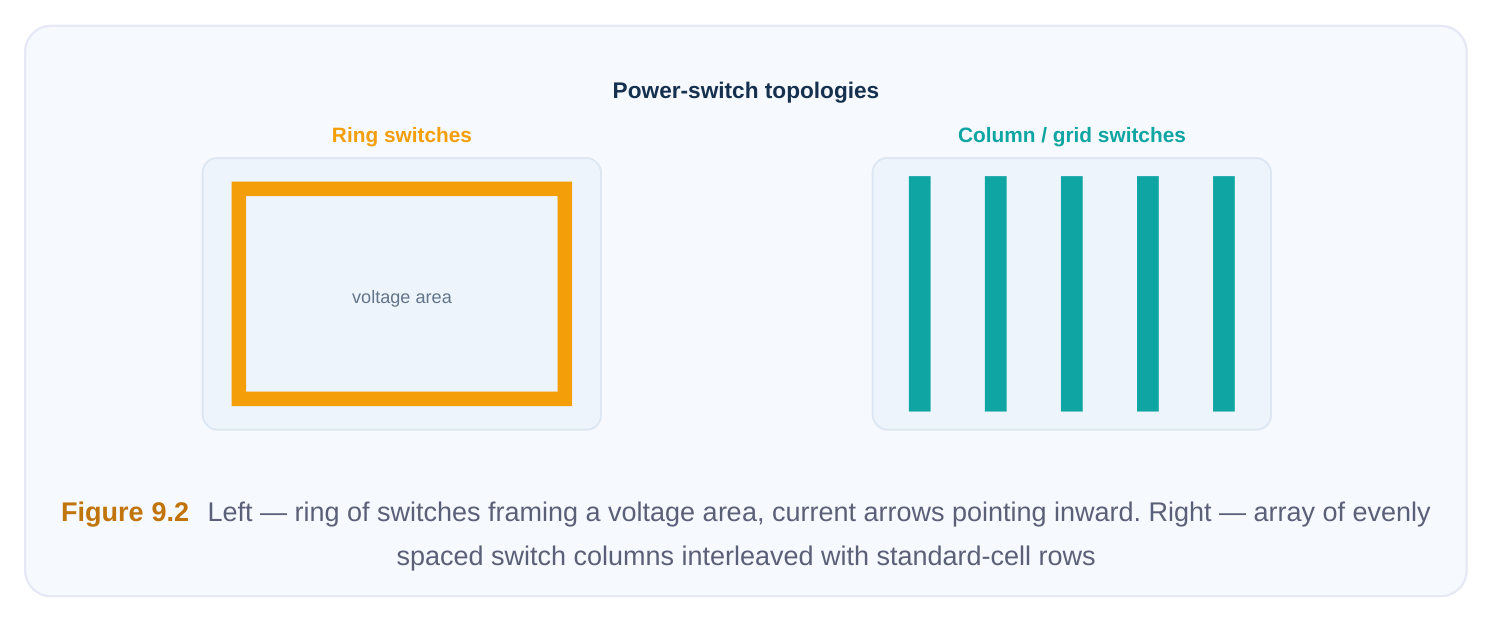
There are two canonical ways to deploy switches, and a mature flow often blends them. Ring switches are placed around the perimeter of a region — typically hugging the boundary of a voltage area. They form a frame that taps the always-on rail on the outside and drives the switched rail on the inside. Rings are clean to route, keep the switch overhead out of the core placement region, and are natural when the gated block is a hard macro-like region whose interior you do not want to disturb. Their weakness is that current has to flow inward from the perimeter, so the center of a large region can be far from the nearest switch and will see more IR drop. Column (in-array / grid) switches are interleaved inside the placement area, usually as periodic columns aligned to the standard-cell rows and the power grid. Because they are distributed throughout the block, they deliver current locally and keep IR drop flat across a large area. The cost is that they occupy core placement sites and must be planned to align with the grid so they do not fight the router.
| Attribute | Ring switches | Column / grid switches |
|---|---|---|
| Placement | Around region perimeter | Distributed inside the array |
| IR-drop uniformity | Worse for large areas (center starved) | Excellent — current sourced locally |
| Core area impact | Low (lives on the boundary) | Higher (consumes placement sites) |
| Routing of enable | Simple loop around the ring | Must thread through every column |
| Best for | Small/medium regions; macro-like blocks | Large flat blocks needing low droop |
| Typical use | Isolated voltage area | Big always-gated logic partition |
Enable buffer styles. The enable signal that turns the switches on is itself a sized net. Two common styles: a buffered enable, where buffers are inserted along the chain to keep the signal sharp across a long string of switches, and a direct (unbuffered) enable for short chains. The buffer style matters because it shapes how steeply each switch turns on, which directly affects inrush — a subject we return to in 9.4.
9.3 Physical Placement Controls
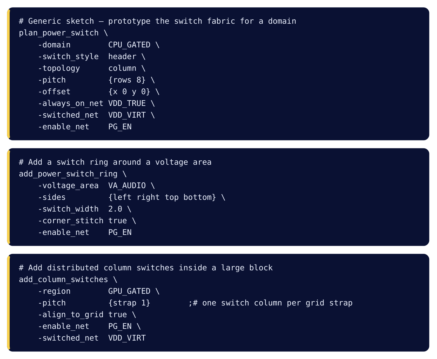
Whatever topology you choose, the switches must land in legal, grid-aligned positions. The planner exposes a handful of controls:
- Switch pitch (spacing). How far apart switches sit. Tighter pitch means more switches per unit area, lower on-resistance, and better droop — at the cost of area. Pitch is usually expressed as a multiple of the cell-row height or the grid strap spacing so switches snap to the power structure.
- Offset. A lateral or vertical shift so the switch cells line up with the always-on straps and the switched-rail straps. Misaligned switches force the tool to detour the rail connection, adding resistance and via count.
- Ring conventions. A switch ring around a voltage area follows the same side/corner conventions as a power ring: you specify which sides get switches, the layer, the width, and how corners are stitched. Consistency here keeps the always-on tap and the switched tap from shorting.
9.4 Sizing the Network and Managing Inrush
This is the analytical heart of the chapter. Two physical effects pull in opposite directions, and the switch count is the single knob that trades between them.
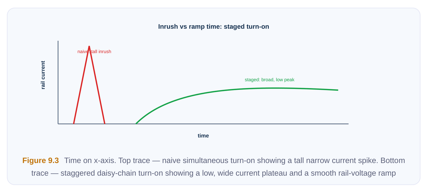
Effect 1 — Steady-state IR drop (the on-state concern). With N switches each of on-resistance R_on sharing the load current I_load, they act roughly as resistors in parallel. The effective series resistance is about R_on / N, and the worst-case rail drop is on the order of I_load × R_on / N. More switches → less drop. This is monotonic and pushes you toward large N. Effect 2 — Inrush / ramp-up current (the wake-up concern). When a gated domain is switched on, its decoupling capacitance and the load capacitance are sitting near zero volts and must charge up to the rail. If you turned every switch on at the same instant, all that capacitance would charge through a very low resistance simultaneously, producing a massive current spike drawn from the always-on grid. That spike causes the always-on rail itself to droop, which can corrupt neighboring always-on logic or retention state. So inrush pushes you toward a gentle, staggered ramp, which often means fewer switches conducting at once, or turning them on one at a time. The reconciliation between these two forces is the enable daisy-chain.
THE ENABLE DAISY-CHAIN
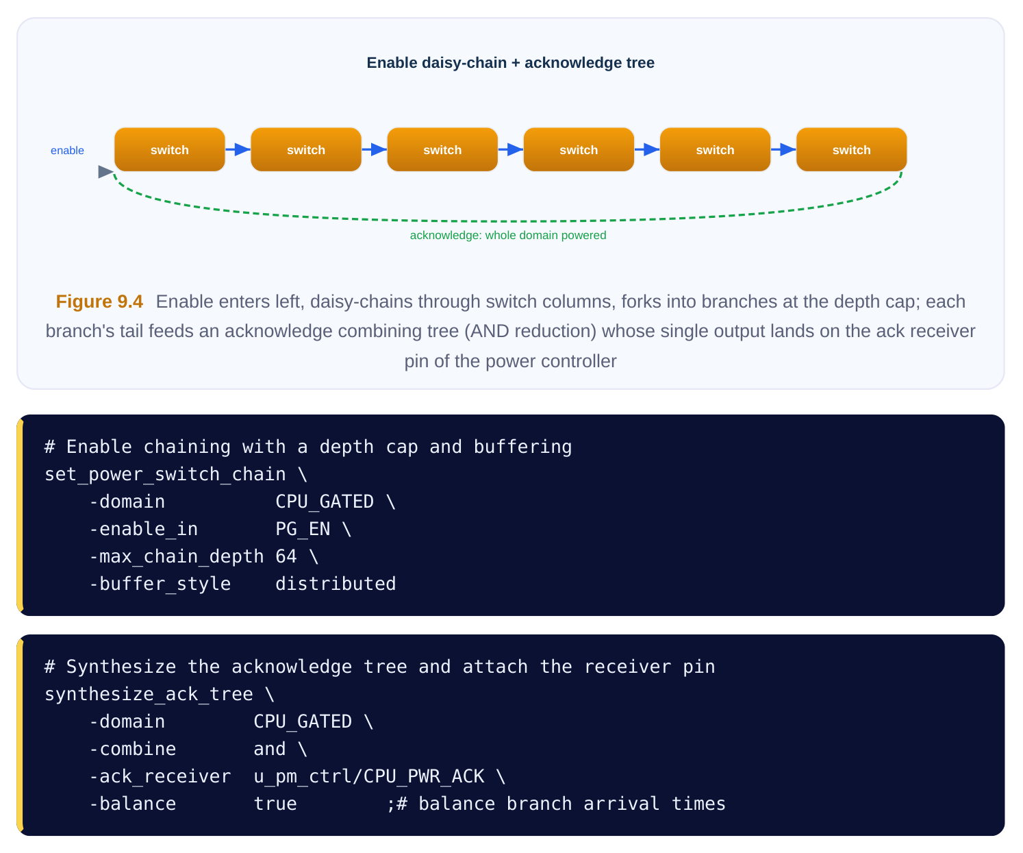
Instead of broadcasting the enable to all switches at once, the enable is threaded from one switch to the next like a shift of activation. Switch 1 turns on, its output enable feeds switch 2 after a delay, which feeds switch 3, and so on. The switched rail charges incrementally. The result is a longer but far gentler ramp, and a much lower peak current. The governing relationships, in plain terms:
- Peak ramp current ∝ (charge to deliver) / (ramp time). Spread the same charge over more time and the peak falls.
- Ramp time ≈ N × (per-stage enable delay). More switches in the chain, or more delay per stage, means a longer total ramp.
- Therefore: for a given maximum allowed inrush current, you can solve for the minimum number of stages (or the per-stage delay) needed to keep the peak under the limit.
This is the switch-enumeration problem: given a peak-current budget, enumerate how many switches and what enable delay deliver a ramp that respects it while still providing enough total oncurrent to meet steady-state IR drop. The optimal switch count is the smallest N that simultaneously (a) keeps steady-state IR drop within budget and (b) keeps inrush within budget — anything beyond that is wasted area and leakage.
| Quantity | Increasing switch count N does... | Driven by |
|---|---|---|
| Steady-state IR drop | Decreases (~1/N) | On-state timing budget |
| Total on-current capacity | Increases | Load demand |
| Off-state leakage | Increases | Power-gating effectiveness |
| Area | Increases | Floorplan budget |
| Ramp-up time (daisy-chained) | Increases | Wake-up latency budget |
| Peak inrush current | Decreases (longer ramp) | Always-on grid robustness |
A clean way to think about it: IR drop and leakage/area set a window (enough switches, but not too many), and inrush sets the chaining strategy (how you turn that fixed N on over time).
9.5 Enable Chaining and the Acknowledge Tree
Once you have decided how many switches and how to stagger them, you have to wire the control. Enable chaining is the act of connecting each switch's enable-out to the next switch's enable-in. The planner controls:
- Maximum chain depth. A single unbroken chain across thousands of switches would have an enormous end-to-end delay and would be impossible to time. So you cap the depth — e.g., "no more than K switches in series before forking." When the cap is hit, the chain forks into parallel branches, trading some ramp uniformity for manageable latency.
- Buffering along the chain. Long chains need buffers so the enable edge does not degrade; this ties back to the enable buffer style of 9.2. The acknowledge (ack) tree. Here is the subtle and frequently-tested part. The enable entering the chain only proves the first switch was told to turn on. The system needs proof that the entire domain is powered before it lets logic run, or before it lifts isolation and de-asserts retention restore. That proof is the acknowledge. The acknowledge is generated at the end of the enable chain (or at the end of every branch) and gathered back through an acknowledge tree — a combining network (typically an AND-style reduction) that asserts only when all branches report "powered." The final combined signal is attached to the acknowledge receiver pin — the input on the power-management controller that waits for it. Only when the ack is high does the controller consider the domain live.
Two interview-grade nuances:
- Why AND-combine? Because power-good is a conjunction: the domain is ready only when every switch leg has turned on. An OR would falsely declare readiness as soon as one leg fired.
- Why balance the tree? So the ack does not arrive skewed; you want it to assert close to when the last leg truly settles, not too early (unsafe) nor wildly late (slow wake-up).
9.6 A Worked Conceptual Planning Example
Consider a gated GPU partition. Assume a load current of about 200 mA in the on-state, a per-switch on-resistance of 5 Ω, an IR-drop budget of 30 mV, and an always-on grid that can tolerate a peak inrush of 80 mA. The numbers below are illustrative, not silicon-accurate — the point is the shape of the trade-off. Step 1 — Switch count from IR drop. Worst-case drop ≈ I_load × R_on / N. To stay under 30 mV: N ≥ (200 mA × 5 Ω) / 30 mV ≈ 33 switches. So the IR-drop floor is roughly 34 switches. Below this, the on-state rail sags too much.
Switch count Approx. effective R Approx. IR drop @200
| N | (R_on/N) | mA | |
|---|---|---|---|
| 16 | 0.31 Ω | ~62 mV | Fails droop budget |
| 34 | 0.15 Ω | ~29 mV | Just meets budget |
| 64 | 0.078 Ω | ~16 mV | Comfortable margin |
| 128 | 0.039 Ω | ~8 mV | Over-provisioned (area/leakage |
waste) Step 2 — Ramp strategy from inrush. Pick N = 64 for headroom. If all 64 turn on at once, the charge dumps fast and peak current blows past 80 mA. Daisy-chaining spreads turn-on over time. Peak current falls roughly as the ramp lengthens.
| Ramp scheme | Ramp time | Approx. peak inrush | Verdict |
|---|---|---|---|
| Simultaneous | ~very short | ~well above 80 mA | Collapses always-on grid |
| Chain, fast per-stage delay | ~medium | ~110 mA | Still over budget |
| Chain, moderate per-stage delay | ~longer | ~75 mA | Meets 80 mA budget |
| Chain, slow per-stage delay | ~longest | ~40 mA | Safe but wake-up too slow |
Step 3 — Topology and enable-chain parameters. The partition is large and flat, so distributed column switches win on IR-drop uniformity. We cap chain depth so the ack does not take forever, then fork.
| Parameter | Chosen value | Rationale |
|---|---|---|
| Topology | Column / grid | Large flat block; need uniform low droop |
| Switch count | 64 | IR margin without leakage/area waste |
| Enable scheme | Daisy-chain, moderate per-stage delay | Inrush under 80 mA |
| Max chain depth | 32 (2 branches of 32) | Keeps end-to-end enable latency tractable |
| Ack combine | AND tree, balanced | Assert only when both branches powered |
| Ack receiver | Power-controller power-good pin | Gates isolation release / retention restore |
The conclusion: 64 switches is the optimal count here — it clears the IR-drop floor of 34 with sensible margin, while staying well under the over-provisioned region where leakage and area begin to dominate. Inrush is then handled entirely by the chaining, not by changing N. That separation — N for droop, chaining for inrush — is the mental model to carry into an interview.
9.7 Interview Q&A
switches are not free. In the off-state they leak, defeating the very purpose of power gating; they consume area and placement sites; and their enable network grows. Past the point where IR drop and inrush are satisfied, every extra switch is pure cost. The goal is the minimum count that meets both the steady-state droop budget and the inrush budget.
decoupling and load capacitance must charge from near zero to the rail. Turning all switches on simultaneously charges that capacitance through a very low resistance at once, producing a current spike large enough to droop the always-on grid and corrupt neighboring logic or retention. The daisychain staggers turn-on so the rail charges incrementally — same total charge, spread over a longer ramp, so the peak current is far lower.
perimeter: clean routing, low core-area impact, good for small or macro-like regions, but the center of a large area can be current-starved and droop. Column switches distribute through the array: they source current locally and keep IR drop flat across a big block, at the cost of consuming placement sites and needing careful grid alignment. Large flat partitions favor columns; compact isolated voltage areas favor rings.
chain was told to turn on. The acknowledge, generated at the chain's end and combined through an AND-style tree, proves that all switches are actually conducting and the domain is fully powered. It lands on the power controller's acknowledge receiver (power-good) pin. Only after the ack asserts should the controller release isolation, restore retention, and let logic run — using a domain before it is fully powered is a functional failure.
IR drop roughly halves (switches act as parallel resistors, ~R_on/N). Off-state leakage and area roughly double. For inrush and ramp it depends on the enable scheme: with a daisy-chain, more stages lengthen the ramp and lower peak inrush; with simultaneous enable, more switches mean a lower-resistance charge path and a higher spike. This is exactly why droop is solved by choosing N, while inrush is solved by choosing how you stagger that N.
Key Takeaways
- The switch fabric is expensive in area, always-on routing, and on-state IR drop — prototype and plan it before full implementation, between floorplanning and grid construction.
- Ring switches suit small/macro-like regions (clean routing, low core impact); column/grid switches suit large flat blocks (uniform low droop) at the cost of placement sites and grid alignment.
- Switch placement is governed by pitch, offset, and ring conventions so switches snap to the always-on and switched rails.
- Sizing is a tug-of-war: more switches → lower IR drop but more area/leakage and longer
chains; fewer switches → smaller but risk droop and a violent ramp.
- Separate the two concerns: pick N from the steady-state IR-drop (and area/leakage) window, then handle inrush via the enable daisy-chain that staggers turn-on and caps peak current.
- The switch-enumeration problem solves, for a given peak-current budget, how many stages and what per-stage delay yield a safe ramp — the optimum is the smallest N meeting both droop and inrush.
- Enable chaining needs a max-depth cap (forking into branches) to keep latency tractable; long chains need buffering.
- The acknowledge tree AND-combines branch tails and lands on the ack receiver pin, confirming the whole domain is powered before isolation release and retention restore.
Comments
Leave a Reply