 ChipBuddy
← Home
ChipBuddy
← Home
Clock Distribution Fundamentals
Clock Distribution Fundamentals
Before any engineer touches a clock optimization engine or argues about skew targets in an interview, they need an honest mental model of why the clock network is unlike every other net in the design. Almost every signal in a chip is a private conversation between a handful of cells. The clock is a public address system: it must reach every sequential element, it switches on a fixed cadence cycle after cycle, and the moment it arrives at each register is the reference against which all setup and hold checks are measured. Get the clock right and the data paths have room to breathe. Get it wrong and no amount of data-path effort will recover the frequency. This chapter builds the vocabulary and the intuition that the rest of the handbook depends on.
Why the Clock Network Is Special
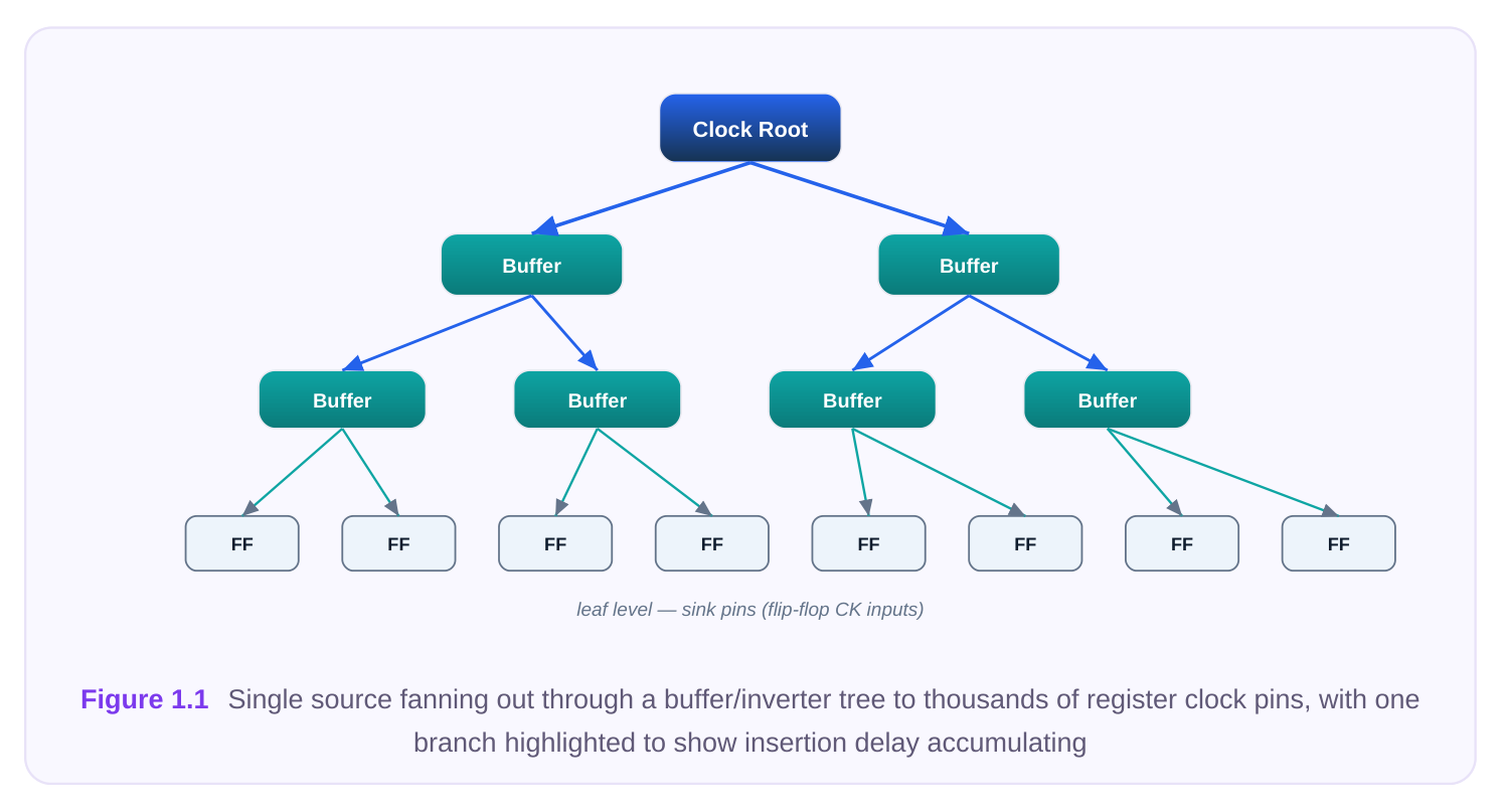
Three properties make the clock distribution network the single most consequential structure in a synchronous design. First, reach. The clock is the only net that, by definition, fans out to the clock pin of every flip-flop and latch in its domain — often hundreds of thousands of endpoints in a modern block. A functional data net might drive a dozen loads; the clock drives an entire population. That fan-out cannot be served by a single driver, so the clock becomes a tree (or a mesh, or a hybrid) of buffers and inverters that physically spans the floorplan. Second, activity. Most logic nets are quiet most of the time; their switching is data-dependent and statistically sparse. The clock toggles every single cycle, twice per period if you count both edges.
High activity multiplied by large total capacitance is exactly the recipe for dynamic power, which is why the clock network routinely consumes 20–40% of a block's dynamic power even though it is a tiny fraction of the cell count. Third, timing leverage. The arrival time of the clock edge at a register is the timing reference. Any imperfection — a late edge, a slow transition, a mismatched path — directly inflates or erodes the timing margin on every path that touches that register. The clock network therefore bounds the achievable frequency and a large slice of the power budget simultaneously.
The Three Governing Metrics
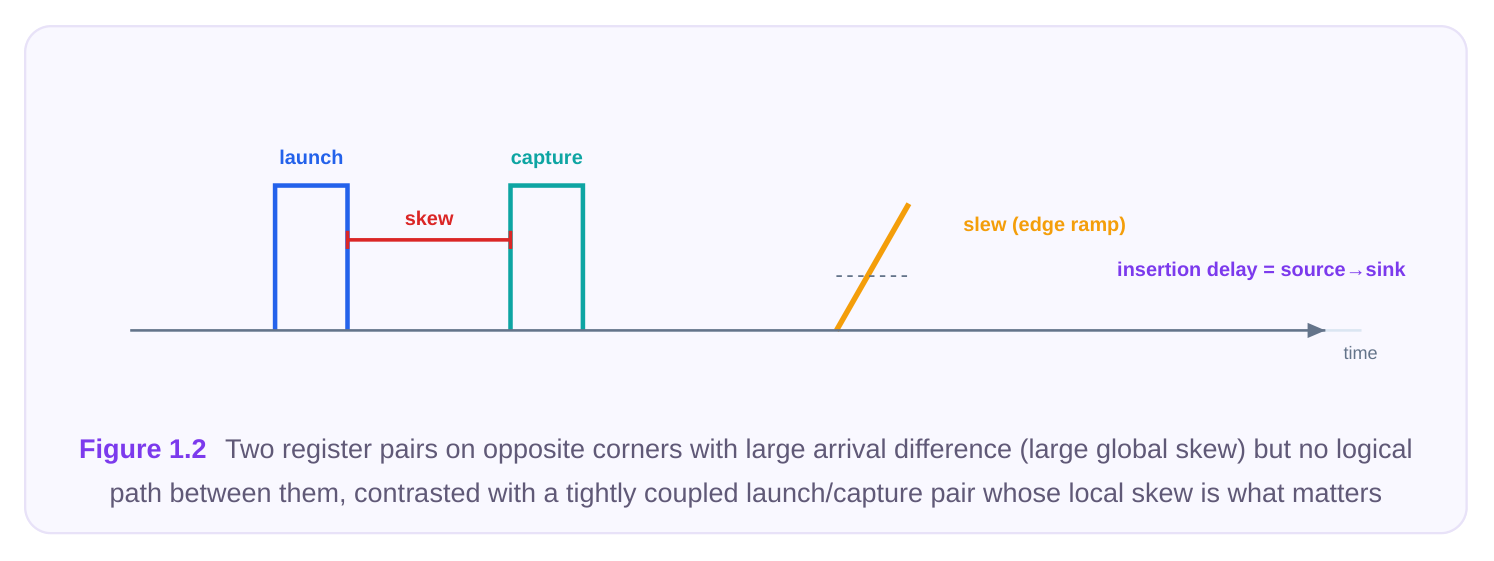
Almost everything you will be asked about clock tree synthesis (CTS) reduces to three numbers. Define them precisely now and the rest of the field falls into place. Clock skew is the difference in clock arrival time between two related endpoints — typically the launching register and the capturing register of a timing path. If the launch flop sees its edge at time t_L and the capture flop sees it at t_C , the skew for that path is t_C - t_L . Skew is a relative quantity: it only has meaning between a pair of sinks that exchange data. A flop on the far side of the chip that never talks to your path is irrelevant to your skew, even if its arrival time is wildly different. Clock slew (also called transition time) is the edge rate of the clock waveform at a pin — how long the signal takes to swing between defined voltage thresholds (commonly 10%–90% or 30%–70%). A clean clock has fast, crisp edges. A degraded slew means the receiving flip-flop's internal timing arc shifts, the effective delay grows, and — critically — slow edges make the cell far more sensitive to noise and to process/voltage/temperature variation. Insertion delay (also called clock latency) is the absolute source-to-sink delay: the time for an edge to travel from the clock source (a port or the root of the tree) to a given register's clock pin. Where skew is a difference between two sinks, insertion delay is the total path length to one sink. Latency comes in
two flavors that interviewers love to separate: network latency (source to register pin, the part CTS builds) and source latency (off-chip or pre-root delay you model but do not build).
| Metric | Precise definition | Primary timing/power effect | Main design lever |
|---|---|---|---|
| Skew | Arrival-time difference between two related sink | Directly adds to/subtracts from setup and hold margin clock pins | Tree balancing, buffer placement, useful-skew scheduling |
| Slew / | Edge rate (time to cross | Slow edges grow effective | Buffer sizing, max-transition |
| transition | voltage thresholds) at a | delay and amplify variation/ clock pin | constraint, drive strength noise |
| Insertion | Total source-to-sink clock | More latency means more | Tree depth, level count, |
| delay / latency | path delay | absolute OCV-induced | target-latency constraint |
uncertainty A subtle but exam-worthy point: skew and insertion delay are not independent. A deep tree (high latency) gives variation more path to act on, which tends to widen the skew distribution even if the nominal balance is perfect. This is why "minimize latency" and "minimize skew" usually pull in the same direction, and why both fight against the noise and variation we discuss below.
How Skew Interacts with Setup and Hold
Skew is not inherently bad — it is signed, and its sign matters differently for the two fundamental timing checks. Consider a launch flop L and a capture flop C, with positive skew defined as the capture edge arriving later than the launch edge. The setup check asks whether data launched on one edge arrives at the capture flop before the next capturing edge. If the capturing edge arrives later (positive skew), the data has more time to settle — positive skew helps setup. The hold check asks whether data does not arrive too early and corrupt the value being captured on the same edge. A later capture edge gives fast new data more chance to race through — positive skew hurts hold. Skew sign (capture relative to
Effect on setup margin Effect on hold margin
| Positive (capture edge later) | Improves (more time to | Degrades (more chance of a |
|---|---|---|
| settle) | race) | |
| Zero (perfectly balanced) | Neutral baseline | Neutral baseline |
| Negative (capture edge earlier) | Degrades (less time to settle) | Improves (harder to race) |
This signed behavior is the entire basis for useful skew, discussed next. The takeaway for now: blindly driving all skew to zero is rarely optimal. Zero global skew is a safe default, but a designer who understands the table above can deliberately push edges around to buy margin where it is scarce.
Useful Skew vs Harmful Skew
The single most important conceptual distinction in this chapter is between skew that is intentional and controlled and skew that is uncontrolled and unknown. Useful skew (sometimes "intentional skew" or, in its scheduled form, the foundation of concurrent clock-data optimization) is a deliberate arrival-time offset inserted to borrow time from a slack-rich path and give it to a slack-poor one. If a path is failing setup, delaying its capture clock (positive skew) hands it extra time — at the cost of the next stage, whose launch edge is now later. Because the offset is chosen by the engine with full knowledge of the timing graph, it is bounded, modeled, and signed off against. Useful skew is a tool. Harmful skew is the uncontrolled spread that arises from imbalanced tree branches, mismatched loads, routing detours, and variation. Nobody asked for it, the timing engine did not plan around it, and it erodes margin on both setup and hold simultaneously because you cannot predict its sign at any given endpoint. Harmful skew is a defect. The same physical phenomenon — a difference in arrival times — is useful when you chose it and harmful when the silicon imposed it on you. The whole discipline of CTS and concurrent clock-data optimization is, in one sentence, maximizing useful skew while minimizing harmful skew.
# Conceptual constraints distinguishing the two regimes.
# A global skew ceiling bounds the harmful spread the tree may produce.
set_clock_tree_options -clock CLK -max_skew 0.040
# A per-path useful-skew budget tells the optimizer it MAY shift
# capture edges within this window to recover setup/hold slack.
set_clock_latency_range -clock CLK -min 0.30 -max 0.45
Local Skew vs Global Skew
Two definitions of skew coexist, and conflating them causes real confusion in reviews. Global skew is the difference between the latest and the earliest arrival times across all sinks in the clock domain, regardless of whether those sinks actually communicate. It is a single, conservative, whole-tree number — easy to report, easy to compare, but pessimistic because it penalizes you for endpoints that never exchange data. Local skew is the skew measured only between related register pairs — flops that are launch/capture partners on real timing paths. This is what actually affects timing closure. Two flops with huge global arrival-time difference but no logical relationship contribute nothing to any setup or hold check between them. Modern flows optimize for local skew (it is what timing cares about) but still report global skew as a sanity metric. An interviewer asking "is 80 ps of skew bad?" is often probing whether you know to ask "global or local, and between which endpoints?"
On-Chip Variation on Long Clock Paths
On-chip variation (OCV) is the reality that two nominally identical buffers, placed micrometers apart, do not have identical delay — because of dopant fluctuation, voltage drop differences, temperature gradients, and lithographic variation. The longer the clock path, the more independent sources of variation accumulate along it, and the wider the resulting uncertainty. This is precisely why insertion delay and skew are linked. A common clock path shared by launch and capture (the segment before the tree branches apart) is common-path pessimism — variation there affects both flops identically and should be credited back. The divergent portion after the branch point is where OCV does its damage: the longer and deeper those divergent segments, the more uncorrelated variation they accumulate, and the more guard-band the timing engine must subtract. Long, deep trees are therefore doubly punished: more latency, and more variation-induced effective skew on top of it. Reducing tree depth and maximizing the common path (a technique known as common-path-pessimism removal, CPPR) are direct responses to this.
# Enable on-chip variation analysis and credit the shared common
# clock path so the timer does not double-count correlated variation.
set_analysis_mode -analysis_type on_chip_variation
set_timing_derate -clock -early 0.95 -late 1.05
set_clock_analysis -common_path_pessimism_removal true
Endpoints: Sinks and Ignore Pins
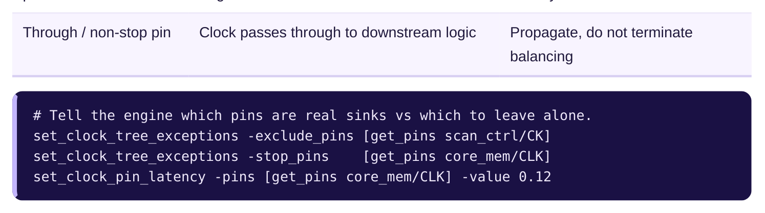
The clock tree's job is to deliver balanced, clean edges to its sinks — the clock input pins of sequential elements (flip-flop and latch clock pins). These are the endpoints the engine balances, the pins where skew and slew are measured, and the loads the buffers must drive. But not every pin reachable through the clock network is a legitimate balance target, and this is a classic interview trap. Ignore pins (or exclude/stop/non-stop pins, depending on the flow's vocabulary) are pins that the clock signal physically reaches but which must not be treated as balancing sinks. Common examples include:
- Clock pins of cells that are functionally on a different domain or are gated off,
- Pins feeding clock-generation or clock-gating logic where balancing would distort the tree,
- The clock inputs of memories or hard macros that carry their own internal latency and must be balanced to the macro boundary, not the internal pin,
- Test or scan-clock pins that are irrelevant in functional mode. If the engine mistakenly tries to balance an ignore pin, it will warp the entire tree to satisfy a constraint that does not matter, burning area and power and potentially worsening the skew on pins that do matter. Endpoint class Role in the clock tree CTS treatment Sink (register clock pin) Real balancing target; skew/slew measured Balance, constrain slew, drive here cleanly Ignore / exclude pin Reached by clock but not a valid balance Stop the tree; do not balance target Macro / memory clock Has internal latency; boundary is the real Balance to boundary, apply pin pin target latency
Why a Clean Clock Costs Area and Power
Here is the trade-off the rest of this handbook spends its time managing. A clock that arrives everywhere with low skew and crisp slew is not free — it is bought with buffers and inverters. To drive a huge fan-out without slew degradation, you insert levels of progressively larger buffers. To balance arrival times across an irregular floorplan, you add delay (more buffers) on the short branches to match the long ones. Every one of those cells occupies silicon area and, far more importantly, switches every cycle, dumping dynamic power into the network. The clock tree is often the largest single contributor to a block's dynamic power precisely because we made it clean. This sets up the central tension of CTS:
- More balancing buffers → lower skew, but more area and more clock power.
- Larger drivers → better slew, but higher switching power and possible electromigration/IR concerns.
- Deeper trees → easier balance over distance, but more latency and more OCV-induced uncertainty.
- Aggressive useful-skew borrowing → recovered timing slack, but a more fragile, harder-to-sign- off tree. Every technique in later chapters — clock gating to suppress unnecessary toggling, mesh and multi- source trees, concurrent clock-data optimization that co-tunes the clock and the logic, and variation- aware sign-off — is ultimately a way to move along these trade-off curves more intelligently than a naive "balance everything to zero skew" approach ever could.
Interview Q&A
one in my path. Is that a skew problem? Not necessarily, and the right answer is to ask whether the two flops are related — that is, whether they form a launch/capture pair on an actual timing path. If they never exchange data, that 200 ps is global skew with no impact on any setup or hold check. Local skew between communicating pairs is what governs closure. This question tests whether you distinguish global from local skew rather than reflexively treating any arrival difference as a defect.
You can deliberately introduce positive useful skew on that path — delay the capture clock so the data has more time to settle, recovering setup margin. The catch is twofold: positive skew degrades the hold check on the same path, and delaying that capture edge also delays the launch edge for the next stage, potentially pushing the problem downstream. Useful skew is a budgeted, signed-off offset chosen by the engine with full timing visibility — not a free lunch.
skew is zero? Because longer, deeper clock paths accumulate more on-chip variation. Two branches that are perfectly matched at nominal can diverge significantly once independent variation acts along their length, and the divergent (non-common) portion of the path is where that uncertainty turns into effective skew the timer must guard-band. Deeper trees also leave less common path to credit back via CPPR. So latency and variation-induced skew rise together — minimizing depth helps both.
balancing a scan-clock pin and a memory's internal clock pin. What went wrong? Those should have been declared as ignore/exclude and stop pins respectively. The scan-clock pin is irrelevant in functional mode and should not be a balance target; the memory pin carries internal latency and must be balanced to its boundary with the internal delay modeled separately, not balanced as if it were an ordinary register sink. By forcing the tree to satisfy constraints on pins that do not matter, the engine distorted branches and burned area and power. Correct sink/ignore-pin declarations are a prerequisite for a sane tree.
Key Takeaways
- The clock network is special because it reaches every sequential element, switches every cycle, and its quality simultaneously bounds the design's maximum frequency and a large fraction of its power.
- Three metrics govern everything: skew (arrival difference between related sinks), slew (edge rate), and insertion delay/latency (total source-to-sink delay). They are coupled — deeper trees raise latency and widen variation-induced skew.
- Skew is signed: positive skew (later capture) helps setup but hurts hold; negative skew does the reverse. Driving all skew to zero is a safe default, not an optimum.
- Useful skew is a deliberate, budgeted offset to borrow time; harmful skew is uncontrolled spread from imbalance and variation. The discipline is to maximize the former and minimize the latter.
- Optimize for local skew between communicating register pairs; report global skew as a sanity check. On-chip variation punishes long, deep clock paths, which is why latency reduction and common-path-pessimism removal matter.
- Balance only true sinks (register clock pins); declare ignore/stop pins so the engine does not warp the tree around pins that do not affect functional timing.
- A clean clock is purchased with buffers and inverters — area and, above all, switching power. Every later technique exists to navigate the skew/slew/latency/power/area trade-offs more intelligently than naive zero-skew balancing.
Comments
Leave a Reply