 ChipBuddy
← Home
ChipBuddy
← Home
Structured Clocks: H-Tree & Multi-Tap
Flow
Most clock trees you will ever build are conventional trees: the synthesis engine starts from a root, grows a buffered network downward toward thousands of sinks, and balances the branches until skew falls within budget. That approach is wonderfully automatic and works for the vast majority of blocks. But there is a class of problems where letting the tool grow an ad-hoc network is simply not good enough — and that is where structured clocking earns its place. This chapter is about deliberately imposing a regular, geometric backbone on the clock before (or instead of) letting an algorithm freely route it. We will cover why structured distribution exists, the flexible H-tree, the multi-tap flow, the idea of building an early clock, and — critically for interviews — when to reach for structure and when to leave it alone.
Why Structured Clock Distribution Exists
A conventional buffer tree balances nominal latency. The trouble is that two branches with identical nominal delay can drift apart dramatically once you account for on-chip variation (OCV), supply droop, temperature gradients, and the random placement of buffers across the die. A long, twisty branch
threaded through congestion sees more variation than a short, straight one — even if the static timing report claims they match. Structured distribution attacks this by making the physical geometry of the network symmetric and predictable. When two paths share the same length, the same number of buffer stages, the same wire width, and the same physical environment, their delays track each other under variation. That tracking is the real prize. You are not just minimizing skew at the nominal corner; you are minimizing how much skew moves across corners, voltages, and ageing.
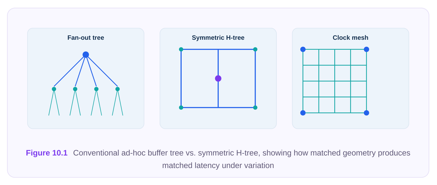
So structured clocking exists for three recurring situations:
- Very low skew targets. When the skew budget is a small fraction of the period, you cannot leave matching to chance.
- High frequency. As periods shrink, the absolute variation budget shrinks with them, so variation tracking matters more than nominal balance.
- Large clock domains. Distributing one clock across a big region means long wires, and long wires are where geometry-driven matching pays off most. Driver Why a conventional tree struggles What structure provides Tight skew budget Branch-to-branch variation dominates the Geometric symmetry keeps branches budget tracking High clock frequency Small absolute jitter/skew margin Predictable, repeatable latency per tap Large physical Long, dissimilar branches diverge under Matched backbone lengths to every domain OCV region Many balanced Tool may balance nominally but not Identical sub-trees by construction replicas physically
The H-Tree Concept
The classic structured network is the H-tree. Starting from the center, you drive two arms; each arm splits into two more arms at right angles, forming an "H"; each of those endpoints splits again, and so on. By construction, every leaf of an ideal H-tree is exactly the same wire distance from the root, through the same number of branch points. Insert a buffer at each branch point and you get matched stage counts as well as matched lengths. The beauty of the ideal H-tree is that insertion delay to every tap is identical by geometry, not by optimization. There is nothing for the balancing algorithm to fix because the structure was symmetric from the start.
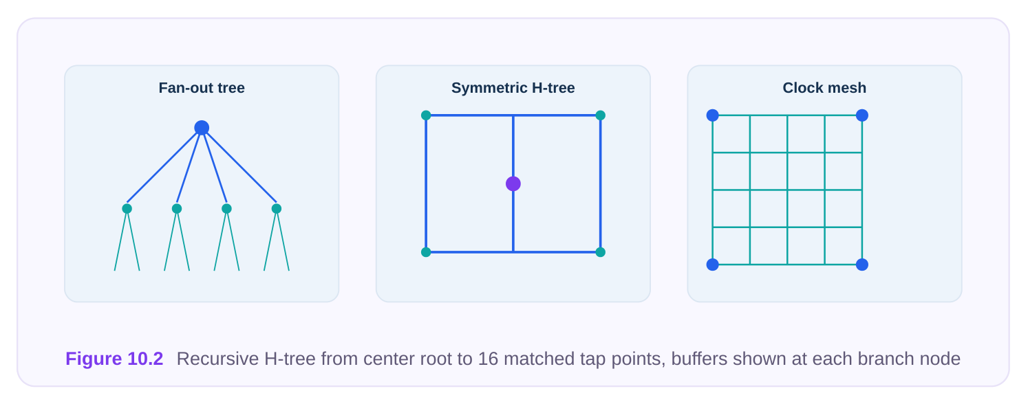
The catch, of course, is that real floorplans are not empty squares. Macros, hard blocks, power straps, keep-out regions, and irregular die outlines all sit exactly where the perfect H wants to route. A textbook H-tree assumes a blockage-free canvas — and you never get one.
Why "Flexible": Blockage-Aware H-Trees
A flexible H-tree is the practical answer. It preserves the intent of the H — matched latency to a set of tap points — while allowing the structure to bend, stretch, and detour around obstacles. Instead of demanding perfect geometric symmetry, the flexible approach matches electrical length: when one arm has to jog around a macro and physically travels farther, the engine compensates the shorter arm (extra wire, tuned widths, or an added stage) so that delay still matches at the taps. The word "flexible" is doing a lot of work here. It means:
- The H can be asymmetric in shape but symmetric in delay.
- Arms can detour around blockages rather than failing or shorting through them.
- Tap points can be placed where the downstream logic actually lives, not where a rigid grid would force them.
- The structure can adapt to a non-square aspect ratio without abandoning latency matching.
You still get the variation-tolerance benefit because the dominant backbone wires are long, wide, straight segments living on upper metal layers, sharing a common environment — even if the overall figure is not a storybook "H".
# Define a flexible, blockage-aware structured backbone
create_clock_structure -type flex_htree \
-clock        CLK_CORE \
-root         clk_root_pin \
-levels       3 \
-route_layers {M7 M8} \
-avoid_blockages true \
-match_latency electrical
# Allow arms to detour but keep matched delay to taps
set_structure_option -structure flex_htree \
-max_detour_ratio 1.4 \
-balance_mode     latency
Multi-Tap Clock Flow
The H-tree gives you matched delay to a set of endpoints, but those endpoints are not the flip-flops — they are tap points. A tap point is where the structured backbone hands off to a conventional local tree that fans out to the real sinks in that region. This two-stage organization is the multi-tap flow. Think of it as a hierarchy of responsibility:
- 1. The backbone (H-tree, spine, or mesh) carries the clock across the die with matched, low-variation
latency to each tap.
- 2. The local trees below each tap do the messy, congestion-aware fan-out to sinks using ordinary
balanced-tree synthesis.
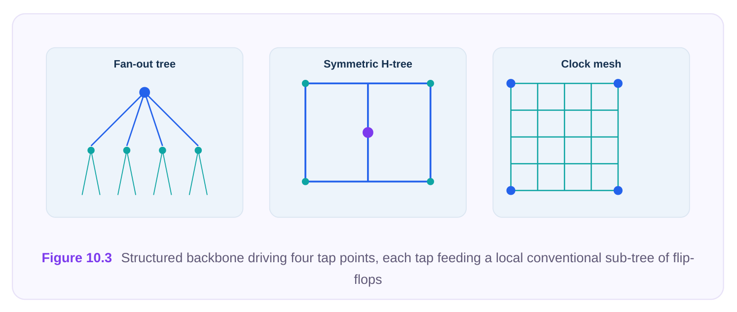
This split is powerful because it isolates the hard problem (long-distance, variation-sensitive distribution) from the easy problem (local fan-out). The backbone handles distance; the local trees
handle density. Two flip-flops in different regions are now only as far apart, electrically, as their two tap points — and the tap points were matched by construction. The job of the flow then becomes balancing across taps. You constrain the insertion delay at every tap point to be equal (or to a defined offset profile), and you constrain each local tree to a target latency from its tap. The total skew between any two sinks is the residual tap mismatch plus the residual local-tree mismatch — each of which is small and bounded.
# Declare tap points on the structured backbone
define_clock_taps -structure flex_htree \
-clock     CLK_CORE \
-tap_pins  {tap_nw tap_ne tap_sw tap_se}
# Force matched insertion delay to every tap
set_tap_constraint -clock CLK_CORE \
-taps         {tap_nw tap_ne tap_sw tap_se} \
-target_latency_match 0.0 \
-tolerance    5ps
# Each tap feeds a conventional balanced local tree
synthesize_local_trees -clock CLK_CORE \
-from_taps    {tap_nw tap_ne tap_sw tap_se} \
-target_skew  10ps
A spine variant works the same way: instead of an H, a wide low-impedance clock spine runs across the block and tap points hang off it at regular intervals. Spines are attractive when the geometry is long and narrow, or when you want the simplicity of a single backbone wire rather than a recursive figure.
Building an Early Clock
One of the most valuable ideas in structured clocking is timing when you build it. The early clock flow constructs a preliminary structured backbone before placement and optimization are final — sometimes right after floorplanning, when only macros and the rough cell distribution are known. Why build a clock you know will change? Because the structured backbone is the part of the clock that is hardest to move later and most disruptive when it shifts. Locking it in early gives you three things:
- Feasibility confidence. You learn immediately whether the floorplan can even host a matched backbone with the available routing layers, or whether macros block the only good arm routes. Better to discover that now than after weeks of optimization.
- Latency budgeting. The backbone fixes the bulk of the insertion delay. Once that number is known, downstream placement and datapath optimization can be done against a stable clock latency rather than a moving target.
- A guide for downstream steps. Tap locations influence where the engine wants to cluster registers, and a known backbone informes useful-skew and concurrent clock-data decisions in later stages.
# Build a preliminary structured clock early, post-floorplan
build_early_clock -clock CLK_CORE \
-type        flex_htree \
-taps_auto   true \
-snap_to     macro_aware_grid \
-estimate_only_local true
# Freeze the backbone; let downstream flows honor it
set_clock_structure_status -clock CLK_CORE \
-backbone fixed \
-local    rebuildable
The discipline here is to fix the backbone but keep the local trees rebuildable. The expensive, matched, upper-metal structure is preserved across iterations, while the cheap local fan-out is regenerated each time placement changes. You get the stability of early commitment without paying for it every time the design churns.
Mesh: The Brute-Force Cousin
For the most aggressive skew targets — top-level clocks on high-performance designs — neither a tree nor an H may be enough. A clock mesh drives a full grid of wire shorted together and fed by many drivers around its perimeter. Because the mesh is one electrically continuous sheet, skew across it is extremely small and remarkably variation-tolerant: a weak driver in one corner is propped up by its neighbors through the shorted grid. The cost is brutal. A mesh shorts together many drivers that fight each other, burning enormous dynamic and short-circuit power, consuming routing tracks, and demanding careful electrical analysis that ordinary tree timing cannot capture. You reach for a mesh only when the skew requirement justifies that expense — typically the highest-frequency global clock on a flagship design, not a routine block.
| Structure | Strength | Primary cost | Typical use |
|---|---|---|---|
| Conventional | Automatic, low resource use, tree | Variation-sensitive over congestion-aware | Default for most blocks long branches |
| Flexible H-tree | Matched, variation-tolerant latency to taps | Extra wire/buffers, planning effort | Large or low-skew domains |
| Multi-tap spine | Simple backbone, easy tap placement | Less symmetric than H, spine loading | Long/narrow blocks, regular tap grids |
| Clock mesh | Lowest skew, best variation tolerance | Very high power, routing, analysis cost | Top-level high-frequency global clocks |
Trade-Offs: When to Use Structure
Structure is not free, and an interviewer will absolutely probe whether you understand the cost. Every benefit of a structured clock has a price tag:
- Area and routing resources. Backbones live on wide upper-metal wires and detour around blockages, consuming tracks that signal routing wanted.
- Power. Wide wires, large backbone buffers, and especially meshes raise clock power — and the clock is already one of the largest power consumers on the chip.
- Effort and rigidity. Planning tap points and freezing a backbone takes engineering time, and a fixed structure is, by design, harder to change when the floorplan shifts. So the decision is a judgment call about whether predictable, variation-tolerant latency is worth those costs. Question Lean conventional tree Lean structured Is the skew budget comfortable? Yes No, it is a tight fraction of the period How large is the clock domain? Small / localized Large, spanning much of the die How high is the frequency? Moderate High, small absolute margin Are routing resources scarce? Yes, avoid heavy Can afford upper-metal backbone backbones Is power the dominant constraint? Yes Skew/robustness outweighs power Does the floorplan have heavy Either, with care Flexible H-tree handles detours blockages? The honest summary: use a conventional tree by default, and escalate to structure only when variation tolerance, skew, or domain size demand it. Structured clocking is a targeted tool, not a starting point. The strongest answer in an interview is not "structured is better" — it is "structured trades power and resources for predictable, variation-tolerant latency, and I'd only spend that budget when the skew or frequency requirement forces my hand."
Interview Q&A
the same nominal skew? Because it matches geometry, not just nominal delay. In an H-tree, paired branches share length, stage count, wire width, and physical environment, so their delays move together under OCV, voltage droop, and temperature. A conventional tree may report identical nominal latency while its branches traverse very different physical environments, so their delays diverge under
variation. The H-tree minimizes how much skew changes across corners, which is what actually breaks timing in high-frequency designs.
flexibility? A textbook H-tree assumes an empty, square canvas and achieves matching through perfect geometric symmetry. Real floorplans have macros, blockages, power straps, and irregular outlines that sit where the ideal arms want to route. A flexible H-tree keeps the intent — matched latency to tap points — but lets arms detour around obstacles and become physically asymmetric, compensating the shorter arms (extra wire, width tuning, or stages) so delay still matches electrically. Without flexibility, the structure would either fail to route or short through blockages.
spine) delivers matched, low-variation latency to a set of tap points; each tap then feeds a conventional balanced local tree that fans out to the real sinks. Total skew between any two sinks is the residual mismatch at the taps plus the residual mismatch within the local trees. You constrain tapto-tap latency to match (within a tight tolerance) and constrain each local tree to a target skew from its tap. Because each component is small and bounded, the overall skew stays controlled — and the hard, variation-sensitive distance problem is isolated from the easy local fan-out.
Because the backbone is the part of the clock that is hardest and most disruptive to move later, while local trees are cheap to regenerate. Building it early confirms feasibility (can the floorplan host a matched backbone on the available layers?), fixes the bulk of insertion delay so downstream optimization works against a stable latency, and guides register clustering and concurrent clock-data decisions. The discipline is to freeze the backbone but keep local trees rebuildable, so you gain stability without re-paying the cost on every placement iteration.
Key Takeaways
- Structured clocking exists to deliver variation-tolerant, predictable latency — it minimizes how much skew moves across corners, not just nominal skew.
- The H-tree achieves matching by geometry: equal length, stage count, and environment to every endpoint. A flexible H-tree preserves matched latency while detouring around real-world blockages and asymmetry.
- The multi-tap flow splits the problem: a matched backbone handles long-distance distribution to tap points; conventional local trees handle dense fan-out. Skew is bounded as tap mismatch plus local-tree mismatch.
- The early clock flow locks in the expensive backbone before final placement to confirm feasibility, stabilize latency budgeting, and guide downstream optimization — backbone fixed, local trees rebuildable.
- Meshes push variation tolerance furthest at the highest power and resource cost, reserved for top- level high-frequency clocks.
- Structure trades area, power, and rigidity for robustness. Default to a conventional tree and escalate to structure only when tight skew, high frequency, or a large domain demands it.
Comments
Leave a Reply