 ChipBuddy
← Home
ChipBuddy
← Home
Reporting in CTS
A clock tree is only as trustworthy as your ability to measure it. You can pour the most elegant constraints into the engine, run a flawless build, and still ship a chip that fails timing in silicon — because the report that would have warned you was never opened, or was read carelessly. Post-CTS reporting is the bridge between "the tool says it's done" and "I can sign this off." This chapter teaches you to read clock-tree reports the way a seasoned physical-design engineer does: not as a wall of numbers, but as a diagnostic instrument that points straight at the problem.
Why Post-CTS Reporting Matters
After clock tree synthesis, the design transitions from ideal clocks (zero-delay, zero-skew abstractions used during placement) to propagated clocks (real buffers, real wires, real delays). Everything downstream — hold fixing, routing, signoff timing — assumes the clock network behaves the way you think it does. If your mental model and the actual tree diverge, you will chase phantom timing violations for days. Reporting exists to close that gap. Before you let the flow advance, you must answer a short list of questions:
- Is global skew within budget, per clock and per corner?
- Are insertion delays (latencies) reasonable and balanced where they need to be?
- Does every clock pin meet the transition (slew) target?
- How deep is the tree, and how many buffers/inverters did it cost?
- For multi-clock designs, are clocks that interact balanced against each other?
- Is dynamic clock power within the budget the architects assumed? If you cannot produce a clean, defensible answer to each, you are not done — you are merely finished running the engine.
The Core Reports and What Each Tells You
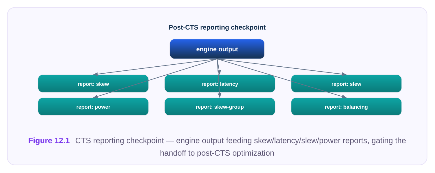
No two flows label these identically, but every mature flow produces the same family of reports. Learn the category and the intent, and you will navigate any tool.
| Report | What it shows | Primary red flag |
|---|---|---|
| Clock-tree summary | Depth, buffer/inverter counts, total clock capacitance, clock power per clock | Excess depth, runaway buffer count, power over budget |
| Per-clock skew | Global (and optionally local) skew for each clock | Skew exceeding the per-clock target |
| Latency / insertion- | Min/max source-to-sink delay; sink-pin latency | Wide min–max spread; latency far |
| delay | spread | above expectation |
| Transition / slew | Slew at clock pins vs. target; count of violators | Any sink over the slew ceiling |
| Skew-group | Skew measured within a defined group of endpoints | Group skew worse than the group's tighter budget |
| Clock-balancing | How interacting clocks are balanced (or | Clocks that should balance are |
| relationships | excluded) | reported as independent |
The clock-tree summary is your first stop — a one-screen vital-signs check. The skew and latency reports tell you whether the tree is balanced and fast enough. The slew report tells you whether the tree is clean (poor edges degrade everything and inflate jitter). The skew-group and balancing- relationship reports matter the moment you have more than one clock that must work together.
Reading a Clock-Tree Report: Key Fields
A typical summary report, stripped to essentials, looks like this:
Clock: core_clk
Sinks ................. 18420
Levels (max depth) .... 11
Clock buffers ......... 1342
Clock inverters ....... 56
Total clock cap (pF) .. 412.7
Max insertion delay ... 0.842 ns
Min insertion delay ... 0.719 ns
Global skew ........... 0.123 ns
Max transition ........ 0.078 ns
Clock power (mW) ...... 38.4
Read it field by field against intent:
| Field | What it tells you | Healthy direction |
|---|---|---|
| Sinks | Number of clocked endpoints driven | Sanity-check vs. expected flop count |
| Levels / depth | Buffer stages root-to-leaf | Shallow as the load allows |
| Buffer / inverter count | Area and power cost of the tree | Proportional to sinks, no surprises |
| Total clock cap | Switched capacitance driving power | Lower is better for power |
| Max / min insertion delay | Latency and its spread | Spread (max−min) drives skew |
| Global skew | Worst arrival difference | Comfortably under target |
| Max transition | Worst clock-pin slew | Under the slew ceiling |
| Clock power | Dynamic power of the network | Within architectural budget |
The deepest insight here: global skew is bounded by the insertion-delay spread. Max delay 0.842 minus min delay 0.719 equals 0.123 — exactly the reported skew. When skew is bad, you look at which sinks sit at the extremes of that spread, not at the skew number itself.
Generic Metric Thresholds
These are starting-point heuristics, not laws. Targets scale with technology node, clock period, and design intent. Use them to know when to worry, then calibrate to your project's signoff constraints.
| Metric | Generic guidance | Interpretation |
|---|---|---|
| Global skew | < ~5–10% of clock period | Higher eats directly into setup/hold |
margin
| Clock-pin | Within library/SDC slew target | Violations degrade delay accuracy and |
|---|---|---|
| transition | add jitter | |
| Tree depth | As shallow as load permits (often single-digit to low teens) | Deeper trees amplify OCV/derate penalties |
| Insertion-delay | Minimize; tighter than skew target | The raw material of skew |
spread
Clock power Within the architectural budget Often a large share of total dynamic A note on depth: every extra buffer stage multiplies the on-chip-variation derate applied to the clock path. A tree two levels shallower frequently shows better signoff skew even when nominal skew is identical, because there is less delay for variation to act on.
Skew Groups and Inter-Clock Balancing
A single global skew number is too blunt for real designs. Two flops on opposite corners of a large die that never communicate do not need to be balanced — forcing them to match wastes buffers and power. Conversely, two register banks feeding the same datapath must be tightly aligned even if the global number looks fine. Skew groups let you scope balancing. You define a group of endpoints that must track one another, and the tool balances and reports skew within that group. Global skew might be 120 ps while a critical skew group is held to 30 ps.
# Define a tightly-balanced group for an interacting datapath
create_skew_group -name dp_align \
-sinks [get_pins {regbank_a/*/CK regbank_b/*/CK}] \
-target_skew 0.030
report_skew_group -name dp_align -format table
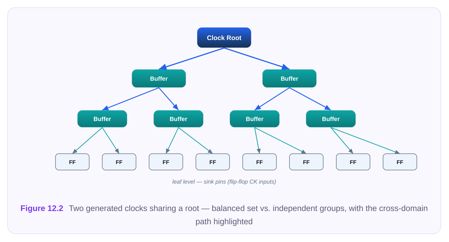
For multi-clock designs, the question becomes how different clocks relate. When data crosses from one clock domain to another with a known phase relationship — divided clocks, or two generated clocks off a common root — the launch and capture trees must be balanced against each other, not just internally. The balancing-relationships report tells you which clocks the engine treated as a balanced set and which it left independent.
# Inspect how clocks were balanced relative to each other
report_clock_balancing -clocks {core_clk core_clk_div2} -format table
The classic failure mode: an engineer assumes the tool balanced core_clk against core_clk_div2 because they share a root, but the report shows them as independent groups. Each is internally tight, yet the cross-domain paths see the sum of two independent insertion delays as skew. The report is where you catch this before timing does.
Tabular vs. Log Output, Filtering, and Spreadsheet Workflows
Reports come in two shapes. Log output is human-readable prose-and-columns, good for eyeballing one clock. Tabular output is machine-parseable — fixed columns, consistent delimiters — and is what you want when scripting, diffing two runs, or loading into a spreadsheet for trend tracking across the project.
# Per-clock skew, filtered to one corner/scenario, in table form
report_skew \
-clock core_clk \
-scenario func_ss_cworst \
-format table > skew_core_clk_ss.rpt
Three habits separate a controlled flow from a chaotic one:
- Filter by clock. Never read all clocks at once on a large design; you will miss the one that matters. Report one clock at a time.
- Filter by corner/scenario. Skew is corner-dependent. A tree balanced at the typical corner can split badly at a worst-case RC corner. Always check the corners that sign off.
- Emit spreadsheet-friendly output. A delimited table per run lets you track depth, skew, and power across iterations and prove you are converging, not thrashing.
| Output mode | Best for | Trade-off |
|---|---|---|
| Log / text | Quick single-clock inspection | Hard to parse or diff at scale |
| Tabular ( -format table ) | Scripting, run-to-run diffs, spreadsheets | Less narrative context |
| CSV / delimited export | Trend tracking, dashboards | Needs downstream tooling |
A simple post-processing pass turns tabular reports into a tracking sheet:
# Loop every clock, dump a uniform table for spreadsheet import
foreach clk [all_clocks] {
report_clock_tree -summary -clock $clk -format table \
>> cts_summary_all_clocks.csv
}
A Worked Interpretation Example
Reports are useless if you cannot turn numbers into a diagnosis. Consider this excerpt from a postCTS skew investigation on core_clk :
Clock: core_clk   (corner: ss_cworst)
Global skew ........... 0.214 ns   (target 0.080 ns)   VIOLATED
Max insertion delay ... 0.961 ns   @ pin  blk_io/sync_reg/CK
Min insertion delay ... 0.747 ns   @ pin  core/alu/acc_reg/CK
Levels (max depth) .... 14
Max transition ........ 0.142 ns   @ pin  blk_io/sync_reg/CK
Clock buffers ......... 1610
Walk it the way you would in an interview:
- 1. Skew is 214 ps against an 80 ps target — a 2.7x miss. Don't panic at the number; find the
extremes.
- 2. The max-delay sink (
blk_io/sync_reg) is also the max-transition sink. That is the tell. A late,
slow-edged sink usually means a long, lightly-buffered wire reaching an isolated endpoint — likely a flop sitting alone near an I/O region far from the clock root.
- 3. Depth is 14, deeper than the rest of the design. The engine added stages chasing that far
endpoint, which simultaneously inflated insertion delay and degraded the edge.
- 4. Min-delay sink sits in the dense core. So the spread is "isolated far sink" vs. "tight core cluster"
— a placement-driven imbalance, not a constraint error. Diagnosis: an outlier endpoint ( blk_io/sync_reg ) is dragging both skew and slew. Fixes, in order of preference: (a) move or cluster the offending flop closer to related logic so the clock reaches it cheaply; (b) if it is a true asynchronous boundary that need not be balanced, place it in its own skew group or exclude it from the balanced set; (c) only as a last resort, let the tool add buffering, which
costs the very depth and power that caused the problem. The report didn't just flag a violation — it named the pin, and the pin named the cause.
Interview Q&A
What's going on? Reported global skew is the worst arrival difference across the whole clock, typically at one analysis condition. Hold violations live on specific launch–capture pairs and are evaluated with on-chip variation: the launch path is sped up by derate while the capture path is slowed, producing an effective skew even when nominal skew is zero. Also, the summary number is often a single corner — hold frequently fails at a fast/best-case corner you didn't report. Re-run skew at the hold-signoff corner and look at the actual path's clock arrivals, not the global figure.
constraints. Where do you look? Depth growth with unchanged constraints almost always means the load the tree must reach changed — usually placement moved sinks farther apart, or a previouslyexcluded set of endpoints got pulled into balancing. Diff the sink count and the max-insertion-delay pin between runs. If a new far-flung pin appears at the latency extreme, the engine added stages to reach it. Check whether placement legalization or an upstream change scattered the flops, and check the balancing-relationships report for newly-included endpoints.
skew over-constrains uncorrelated endpoints and under-protects correlated ones. Flops that never interact don't need to match, and forcing them to wastes buffers and power; flops feeding a shared datapath need tighter balancing than the global budget. Skew groups let you set a strict target on the paths that matter and a relaxed one elsewhere, and the per-group report proves each critical interaction is held — something a single global number can hide.
quality is foundational. A degraded clock edge makes delay calculation less accurate, increases susceptibility to noise and on-chip variation, and contributes to jitter — all of which erode real timing margin that the nominal skew number doesn't capture. Worse, a slow edge on a deep path is often a symptom of an under-buffered or over-long route that will also widen insertion-delay spread. Fixing the transition usually improves skew robustness as a side effect, so it is never "just" a slew issue.
Key Takeaways
- You cannot sign off a clock you cannot measure; post-CTS reporting is the gate between "engine finished" and "I trust this tree."
- The core report family is universal: tree summary, per-clock skew, latency/insertion-delay, transition/slew, skew-group, and inter-clock balancing — learn the intent of each, not one tool's labels.
- Global skew equals the insertion-delay spread; when skew is bad, hunt the min and max sinks, not the skew number.
- Tree depth multiplies variation penalties — a shallower tree often signs off better even at equal nominal skew.
- Use skew groups to balance what interacts and leave the rest free; for multi-clock designs, always verify the balancing-relationships report so cross-domain clocks aren't silently treated as independent.
- Always filter reports by clock and by corner/scenario, and emit tabular/spreadsheet-friendly output so you can track convergence run-to-run.
- A good report names the pin; the pin names the cause. Read reports to diagnose, not just to confirm.
Comments
Leave a Reply