 ChipBuddy
← Home
ChipBuddy
← Home
The CTS Flow & Quick Start
Chapter 4 — The CTS Flow & Quick Start
Clock tree synthesis (CTS) is one of those steps that looks deceptively simple from the outside — "just buffer the clock" — but in practice it is the hinge on which the entire timing closure of a block swings. Get it right and the rest of the implementation flow glides; get it wrong and you spend weeks chasing skew, hold violations, and IR-droop-induced jitter that no amount of routing effort will fix. This chapter walks the end-to-end flow at a practical level: what must be true before you start, the smallest correct recipe to grow a first clock tree on a brand-new design, what the engine is actually doing under the hood, where concurrent clock-data optimization (CCD) plugs in, and how to read runtime so you can plan your iterations. Treat it as the chapter you re-read the night before you run CTS on an unfamiliar block.
Where CTS Sits in the Flow
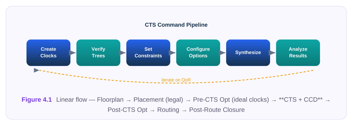
CTS is a midpoint, not a beginning. By the time you launch it, placement has already committed every register and most of the combinational logic to legal locations, and the data-path optimizer has done a first pass on setup timing with ideal clocks — clocks treated as zero-delay, zero-skew nets. CTS replaces that fiction with real, physical buffer trees, and in doing so it changes every clock arrival time in the design. That single fact explains most of CTS's reputation: every downstream number (skew, insertion delay, hold slack, even some setup paths) is meaningless until the tree is built.
PREREQUISITES — THE FOUR GATES
Do not run CTS until all four of these are genuinely true. Skipping any one of them is the most common cause of a "bad" clock tree that is really just garbage-in.
- 1. Placement is legal and stable. Cells sit on rows, no overlaps, and the placement is not going to
be re-shuffled. CTS builds geometry around fixed register locations; if placement moves later, your tree is stale.
- 2. Clocks are fully defined. Every
create_clockandcreate_generated_clockexists, and the
clock relationships (synchronous groups, async groups, physically exclusive) are declared. The engine balances what you tell it about — undeclared generated clocks become unbalanced surprises.
- 3. Constraints are clean. Reasonable I/O delays, declared false paths and multicycle paths, and any
clock uncertainty/jitter budgets. Garbage exceptions cause the optimizer to over- or under-fix paths.
- 4. Power infrastructure is ready. The power grid is built and the rails the clock buffers will tap are
real. Clock buffers switch hard and often; if you build a tree before the grid exists, your post-CTS IR and EM analysis is fiction. The following table is the mental checklist I run through before every CTS launch.
| Gate | What to verify | Symptom if skipped |
|---|---|---|
| Placement legal | No overlaps, density sane, registers | Buffers placed in illegal spots; tree re-builds |
fixed
| Clocks defined | All real + generated clocks, groups | Unbalanced generated clocks, missing skew |
|---|---|---|
| declared | groups | |
| Constraints | I/O delays, false/multicycle paths, | Over-fixing, wasted buffers, wrong latency |
| clean | uncertainty | targets |
| Power ready | Grid built, rails reachable | Fake IR/EM, late surprises in signoff |
The Quick-Start Recipe
When you land on a brand-new block and just need a first clock tree to look at — something to sanitycheck the flow and get real numbers — resist the urge to specify everything. The fastest path to a reasonable first tree is to give the engine clean inputs, a short list of safe buffer/inverter cells, sane targets, and let it run on default effort. Refinement comes later. Here is the smallest correct sequence. The command names below are generic; your tool will spell them differently, but the shape of the flow is universal.
# --- Quick-start CTS recipe (minimal, brand-new design) ---
# 1. Confirm the design is in the right state
check_design_state            ;# placement legal? clocks defined? power built?
report_clocks                 ;# eyeball every clock + generated clock
# 2. Tell the engine which library cells it may use
set_cts_buffer_cells   {BUFx4 BUFx8 BUFx16}
set_cts_inverter_cells {INVx4 INVx8 INVx16}
# 3. Set a few sane targets (units illustrative)
set_cts_target -max_skew      50ps
set_cts_target -max_latency   600ps
set_cts_target -max_transition 100ps
# 4. Build the tree
synthesize_clock_tree
# 5. Look at what you got
report_clock_tree -summary
Three habits make a quick start trustworthy. First, keep the cell list short — a handful of drive strengths of one buffer and one inverter family. A bloated list slows the engine and rarely improves the tree on a first pass. Second, set targets that are achievable, not aspirational: a too-tight skew target makes the engine thrash and burn buffers. Third, always read the summary before you touch anything. The first tree tells you whether your inputs were sane.
ITERATING FROM THE FIRST TREE
Once you have numbers, iterate deliberately. Change one thing at a time so you can attribute cause to effect:
- Skew too high? Loosen nothing yet — first check whether the high skew is on a path you actually care about (CCD may resolve it cheaper than a tighter target). Then consider a tighter
-max_skewor enabling useful skew. - Latency too high? Trim the cell list to stronger drivers, or relax
-max_latencyif the absolute number doesn't matter and only skew does. - Transition (slew) violations? Add a stronger drive-strength cell or tighten
-max_transition; slew fixing is usually a cell-list problem.
- Buffer count exploding? Your skew target is probably too tight, or the engine is fighting a placement problem (registers clustered far from their source).
What the Engine Does Internally
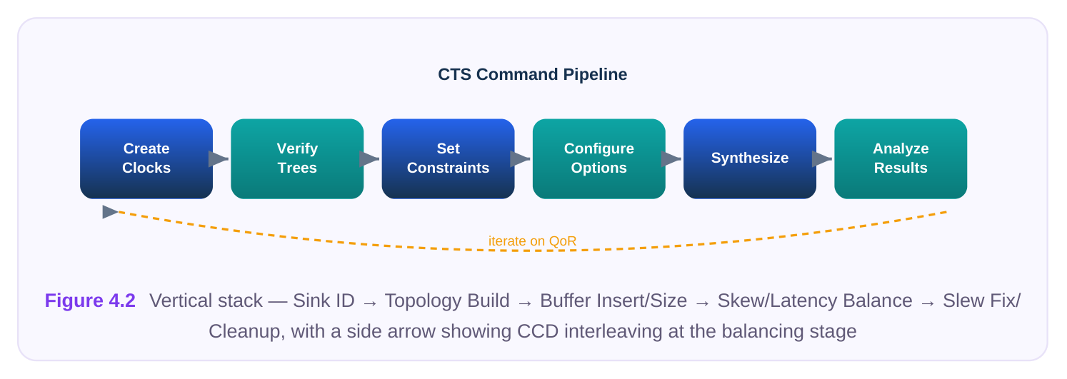
Understanding the internal stages turns CTS from a black box into something you can debug. At a high level the engine moves through five conceptual phases. They are not always cleanly separated in the tool, and CCD interleaves with several of them, but thinking in these terms helps you reason about logs and reports.
- 1. Endpoint (sink) identification. The engine traces from each clock source through the design and
collects every clock pin it must drive — register clock pins, gating cell inputs, macro clock ports, and the boundaries where one clock hands off to a generated clock. These become the sinks of the tree. Anything mis-identified here (a wrong clock definition, an undeclared generated clock) poisons everything downstream.
- 2. Topology construction. Given the set of sinks and their physical locations, the engine builds a
tree structure — deciding clustering, branch points, and the rough shape (a classic balanced tree, an H-tree-like structure for regularity, or a mesh/hybrid for very tight skew). This is where the geometry of placement directly shapes the result.
- 3. Buffer insertion and sizing. The engine populates the branches with buffers and inverters from
your cell list, choosing drive strengths to meet load and transition targets at each level. Inverter pairs are often preferred because they give cleaner duty-cycle behavior and tighter slew control.
- 4. Skew and latency balancing. Now the engine equalizes arrival times across sinks, adjusting
buffer levels and sometimes detouring nets to add delay to fast branches. This is the heart of CTS and where the skew/latency targets actually bite.
- 5. Slew (transition) fixing and cleanup. A final pass repairs any remaining transition or capacitance
violations, legalizes inserted buffers, and tidies the tree.
| Internal stage | What it decides | Knob that influences it |
|---|---|---|
| Sink identification | Which pins are tree leaves | Clock definitions, exclusions |
| Topology construction | Tree shape, clustering | Structure style, NDR rules |
| Buffer insert/size | Drive strength per level | Buffer/inverter cell list |
| Skew/latency balance | Arrival-time equalization | Skew/latency targets, useful skew |
| Slew fixing | Transition repair | Transition target, cell list |
Where Concurrent Clock-Data Optimization Plugs In
Classic CTS balances the clock tree in isolation — it tries to make every clock arrive at the same time, then hands off to the data-path optimizer to fix whatever setup/hold problems remain. That is leaving timing on the table. Concurrent clock-data optimization (CCD) instead optimizes the clock tree and the data paths together: rather than forcing zero skew, it deliberately schedules clock arrivals — pushing a capturing register's clock slightly later to give a critical setup path more time, or pulling it earlier to relieve a hold issue. This is "useful skew" applied at scale and solved jointly with sizing and buffering of the data path. In the flow, CCD lives inside the CTS step (or immediately fused with it), not after. The engine builds the tree while it is already aware of data-path slack, so the topology and the skew schedule are codesigned. Enabling it usually looks like flipping a mode on before you synthesize.
# Enable concurrent clock-data optimization before building the tree
set_cts_mode -ccd true
set_cts_mode -ccd_optimize_setup true
set_cts_mode -ccd_optimize_hold  true
synthesize_clock_tree         ;# tree + skew schedule co-optimized
report_timing -setup -hold    ;# CCD should have improved both
The practical payoff: CCD typically recovers setup slack on the worst paths "for free" (no extra datapath cells) by borrowing time through skew, and it heads off hold problems before routing instead of after. The trade-off is that the resulting skew is no longer near-zero by design — your skew report will show intentional non-zero values, and that is correct. Do not "fix" useful skew by tightening the skew target; you will throw away exactly the optimization you wanted. Read CCD's effect in the timing reports, not the skew report.
Runtime Expectations and Effort
CTS runtime scales with sink count, clock count, and effort level — and CCD adds to it because the engine is solving a bigger joint problem. As a rough mental model: a small block (tens of thousands of sinks) on default effort is minutes; a large block (hundreds of thousands of sinks) with high-effort CCD can be hours. The effort knob is the main lever.
| Effort | Roughly what it does | Runtime | When to use |
|---|---|---|---|
| Low / fast | Coarse balancing, light optimization | Fastest | First sanity tree, flow bring-up |
| Medium (default) | Balanced quality vs. time | Moderate | Most iterations |
| High | Aggressive balancing + full CCD | Slowest | Final/near-signoff runs |
The discipline that saves the most wall-clock time: run low effort first to validate inputs (right cells, right targets, sane sink count), confirm the tree is structurally healthy, then turn up effort for the run whose numbers you'll actually trust. Running high effort on bad inputs just makes you wait longer to discover the inputs were bad.
# Effort progression across a session
set_cts_mode -effort low
synthesize_clock_tree              ;# fast — validate inputs
report_clock_tree -summary
set_cts_mode -effort high -ccd true
synthesize_clock_tree              ;# trusted run
report_clock_tree -summary
report_timing -setup -hold
The Stage Table — Whole Flow
This is the end-to-end CTS flow as a single reference. Each row is a stage you can checkpoint and verify before moving on.
| Stage | Action | Output | Check |
|---|---|---|---|
| Pre-flight | Verify placement, clocks, constraints, | Go/no-go decision | All four gates pass |
power
| Setup | Define cell lists + targets, enable CCD | CTS configuration | Cells exist; targets achievable |
|---|---|---|---|
| Synthesis | Build the clock tree (+CCD) | Buffered clock tree | Tree built, no errors |
| Analysis | Report skew, latency, slew, timing | QoR numbers | Targets met; useful skew sane |
| Iterate | Adjust one knob, re-run | Improved tree | Trend in right direction |
| Handoff | Lock tree, prep for routing | Routable clock nets | Tree marked, NDRs set, no DRCs |
Post-CTS Handoff to Routing
When the tree is good, prepare it for routing. Clock nets are special: they typically get non-default routing rules (wider wires, extra spacing, shielding) so the carefully balanced delays survive real
routing parasitics. Mark the clock nets, apply the routing rules, and run a post-CTS optimization pass that re-times the design with the now-real clock before routing commits.
# Post-CTS handoff
report_clock_tree -summary           ;# final QoR snapshot
set_clock_routing_rule -shield true -width 2x
optimize_design -post_cts            ;# re-time with real clock, fix hold
check_clock_tree                     ;# DRC/structural sanity before routing
The single most important post-CTS check is hold timing. Once clocks are real, hold violations that were invisible under ideal clocks appear; the post-CTS optimization pass should fix the bulk of them so routing starts from a clean state.
Quick-Start Checklist
- [ ] Placement legal and frozen
- [ ] Every clock and generated clock defined; groups declared
- [ ] Constraints clean (I/O delays, false/multicycle paths, uncertainty)
- [ ] Power grid built and reachable by clock buffers
- [ ] Short, sane buffer + inverter cell list set
- [ ] Achievable skew / latency / transition targets set
- [ ] First tree built at low effort; summary read
- [ ] CCD enabled for the trusted run
- [ ] Skew read in timing reports, not fought in the skew report
- [ ] Post-CTS hold fixed; clock NDRs applied before routing
Interview Q&A
around the fixed locations of clock sinks. If placement changes afterward, every register moves, the geometry the tree was balanced for is gone, and your skew/latency are invalid. Placement must be legal and stable so the tree is built against locations that won't shift.
zero skew. What do you tell them? That this is expected and desirable. CCD intentionally schedules clock arrivals — useful skew — to borrow time for critical setup paths and relieve hold paths. The nonzero skew is the optimization working, not a bug. They should evaluate success in the setup/hold timing reports. Tightening the skew target to force zero skew would destroy exactly the slack CCD recovered.
do you debug it? Start with inputs, not knobs. Check whether the skew target is unrealistically tight — that's the classic cause of buffer explosion as the engine thrashes to equalize. Then check the cell list (too weak drivers force more levels). Then look at placement: registers clustered far from their clock
source force long, deep trees. Fix the root cause rather than just relaxing the latency target, which only hides it.
first to validate that inputs are correct — right cells, achievable targets, sane sink count, structurally healthy tree — because that pass is fast and exposes input errors cheaply. Only after the inputs check out do you run high effort with full CCD for the numbers you'll actually trust. This avoids spending hours on a high-effort run that fails because of a problem a one-minute low-effort run would have caught.
Key Takeaways
- CTS is a midpoint that replaces ideal clocks with real buffer trees, invalidating all prior clock- dependent numbers — treat post-CTS reports as the first real timing picture.
- Never launch CTS until the four gates pass: legal placement, fully defined clocks, clean constraints, and a built power grid.
- The quick-start path is a short cell list, achievable targets, a low-effort first build, and reading the summary before changing anything.
- Internally the engine moves through sink identification, topology build, buffer insertion/sizing, skew/ latency balancing, and slew fixing — knowing these stages makes logs debuggable.
- CCD lives inside CTS and co-optimizes clock and data by scheduling useful skew; judge it in timing reports, and never fight intentional skew by tightening the skew target.
- Use low effort to validate inputs and high effort for trusted runs; hand off to routing only after hold is fixed and clock non-default routing rules are applied.
Comments
Leave a Reply