 ChipBuddy
← Home
ChipBuddy
← Home
Executing synthesize_clock_trees
When you have finished configuring your clock specifications, root pins, non-default routing rules, target skew, and buffer/inverter library cells, everything funnels into a single command: synthes‐ ize_clock_trees . This is the moment the tool stops reading your intent and starts building physical structure on the die. Understanding what happens during that run — what the tool does second by second, how long it should take, how to read the console, and what to do when it stalls — separates an engineer who simply launches CTS from one who can steer it. This topic walks through the execution of synthesize_clock_trees end to end.
10.1 Command Syntax
The single most surprising thing about synthesize_clock_trees to a newcomer is how little you actu‐ ally type. In its most common form, the entire invocation is:
synthesize_clock_treesThat is it. There are no mandatory positional arguments and no required options. This is deliberate. By the time you reach this step, you have already told the tool everything it needs through the configura‐ tion state of the design and the CTS specification you loaded earlier. The command is a trigger, not a parameter dump.
What does the tool consult to figure out its parameters? It pulls from several places that were set up before this point:
- The clock definitions in your timing constraints (
create_clock,create_generated_clock) tell it which networks exist and where they originate. - The CTS specification or clock-tree options object holds your targets for skew, maximum latency, transition (slew), and capacitance.
- The list of buffer and inverter cells you marked as usable for the clock network.
- Non-default routing rules (NDRs) and routing layer preferences attached to clock nets.
- The current legalized placement and the floorplan, which define where things physically sit. Because the command reads this accumulated state, two engineers can type the identical command and get completely different trees — the difference lives entirely in the setup. You can pass optional ar‐ guments to override behavior for a single run (for example, restricting synthesis to a specific clock or set of corners), but the philosophy of the command is "configure once, execute simply."
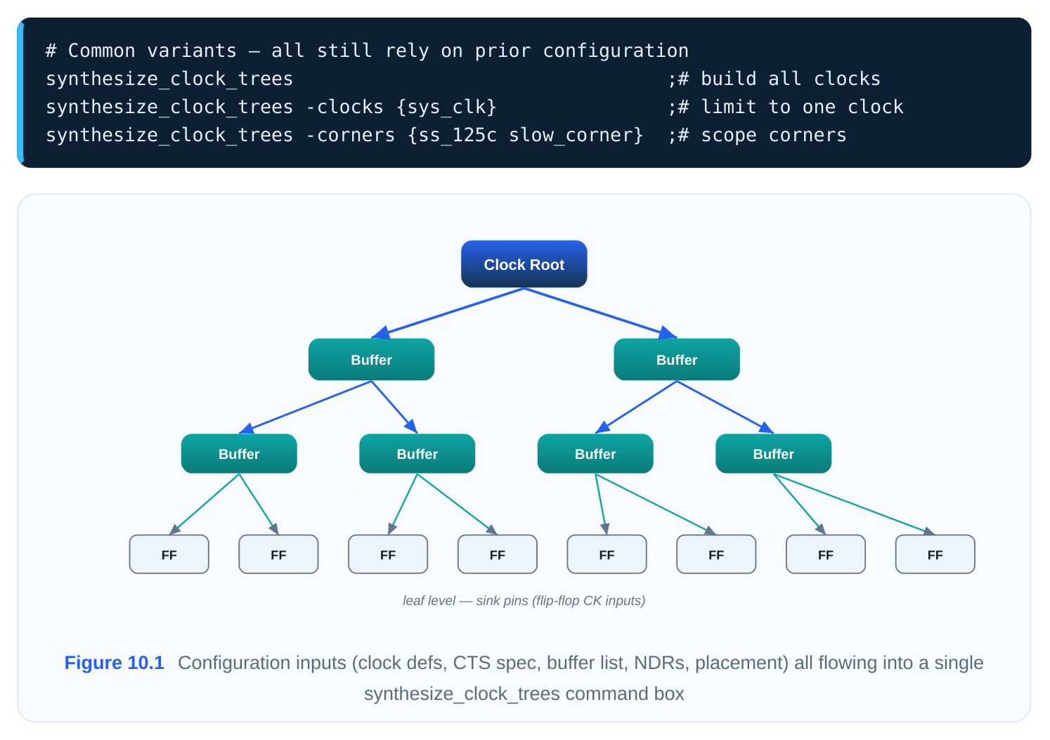
A useful mental model: think of the command like pressing "Render" in a 3D application. The render button has no arguments because the scene, lighting, and camera are already defined. CTS works the same way — the scene is your design state.
10.2 Execution Phases
When the command launches, it does not do its work in one undifferentiated blob. It marches through a recognizable sequence of internal phases. The exact phase names vary by tool vendor, but the stages are universal because they reflect the fundamental problem CTS solves: find the sinks, decide a structure, make it legal, then make it fast and balanced. The timing ranges below are representative for a moderate block; large or congested designs scale up considerably.
| Phase | Name | Typical Window | What Dominates |
|---|---|---|---|
| 1 | Endpoint Identification | 0–4 s | Tracing nets, collecting sinks |
| 2 | Topology Creation | 4–18 s | Choosing tree structure |
| 3 | Legalization | 18–55 s | Placing buffers without overlap |
| 4 | Timing Optimization | 60–300+ s | Sizing, balancing latency, fixing skew/slew |
| 5 | Reporting | a few s | Writing metrics and logs |
Phase 1 — Endpoint Identification (0–4 s)
The first job is to figure out what the tree must drive. Starting from each clock root pin, the tool traces forward through the netlist, following the clock signal until it reaches every termination point — the clock pins of flip-flops, latches, integrated clock-gating cells (ICGs), macro clock inputs, and any explicitly defined clock outputs. These termination points are the sinks (also called clock endpoints or leaf pins). During this pass the tool also classifies special structures. A clock-gating cell, for example, is both a sink (its own clock pin must be driven) and an intermediate node (its output continues the clock further downstream). The tool builds an internal map of the clock's logical reach and marks any non-stop or exclude pins you specified. This phase is fast — usually only a few seconds — because it is essen‐ tially graph traversal with no physical optimization yet. If this phase reports far fewer or far more sinks than you expect, that is your earliest signal that a constraint or exception is wrong.
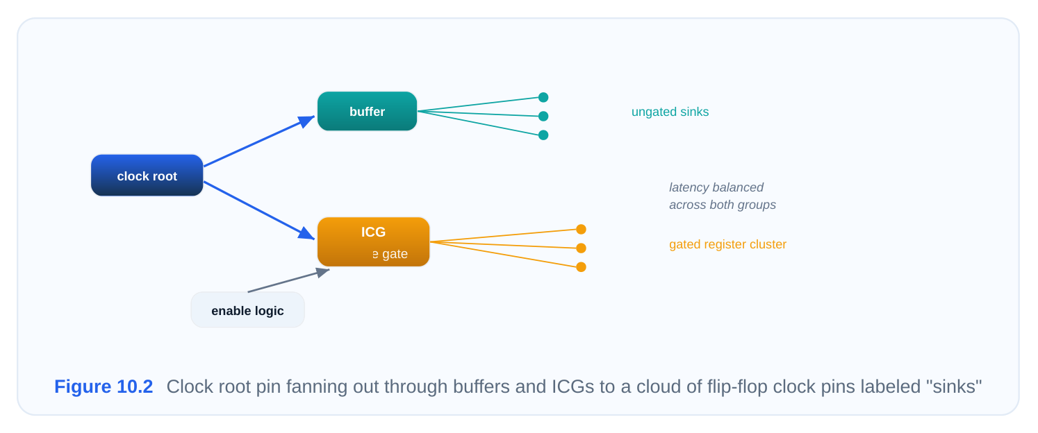
Phase 2 — Topology Creation (4–18 s)
Now the tool decides how to connect the root to all those sinks. This is where the architectural choice between a structured H-tree and a custom (clustered) topology matters. An H-tree lays out the clock distribution as a recursive, geometrically balanced pattern — branches split symmetrically so that the wire length from the root to any sink is, by construction, nearly identical. H-trees are excellent for inherently low skew and are common for top-level clock spines and very regular sink distributions. Their weakness is that real designs rarely have uniformly placed flip-flops, so a pure H-tree can waste buffering and routing on sparse regions. A custom topology (the default for most automatic CTS engines) instead clusters sinks by proximity and balances the tree based on the actual placement of registers. The tool groups nearby sinks under shared driver buffers, then balances those clusters upward toward the root. This adapts to irregular layouts and usually produces less buffer area than forcing an H-tree onto a non-uniform design. Most flows let you mix the two — an H-tree backbone feeding clustered sub-trees. In this phase the tool produces a logical tree: it knows the branching structure and roughly how many buffer levels it needs, but it has not yet committed every buffer to a legal coordinate. Topology creation is more expensive than endpoint identification because it involves clustering heuristics, but it is still typically under half a minute for a moderate block.
Phase 3 — Legalization (18–55 s)
A logical tree is useless if its buffers sit on top of standard cells or on each other. Legalization is the phase that gives every clock buffer and inverter a real, non-overlapping location on the placement grid, snapped to legal sites and rows. Two pressures fight here. First, overlap avoidance: each newly inserted buffer must find an empty legal site, which may force it away from its electrically ideal position. Second, congestion avoidance: dumping a column of buffers into an already-dense region creates routing hotspots, so the legalizer spreads them out and may shove surrounding logic to make room. The tool tries to keep buffers close to their intended branch point while respecting placement density and blockages. In congested
designs this phase balloons, because the legalizer has to search farther for open sites and may need several passes of local cell shuffling.
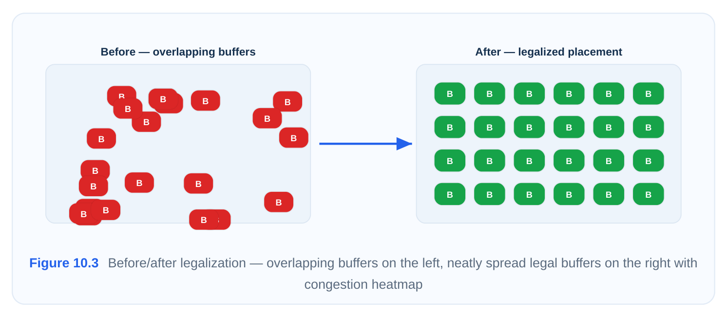
Phase 4 — Timing Optimization (60–300+ s)
This is the longest and most computationally heavy phase, and it is where CTS earns its name. With a legal physical tree in place, the tool now iterates to hit your electrical and timing targets. Four activities interleave here:
- Buffer sizing — swapping each buffer/inverter for a stronger or weaker variant from your allowed cell list so that drive strength matches the load it sees.
- Insertion-delay balancing — adjusting the path from root to each sink so all sinks receive the clock edge at nearly the same time. The tool may add delay buffers to short branches or restructure long ones.
- Skew minimization — driving the spread of arrival times across sinks down toward your skew target, including handling clocks that interact at the same registers.
- Slew (transition) and capacitance fixing — ensuring every clock pin sees a transition edge sharp enough to meet your max-transition rule and that no net exceeds max-capacitance, which usually means inserting more buffers or upsizing existing ones. These goals trade off against each other, so the engine loops: size, re-evaluate timing, re-balance, re- check slew, repeat. Each loop costs real CPU time, especially when analysis runs across multiple corners and modes (MMMC). This is why the phase has such a wide window — a clean design con‐ verges in a minute or two, while one fighting tight skew or aggressive slew rules across many corners can run for many minutes.
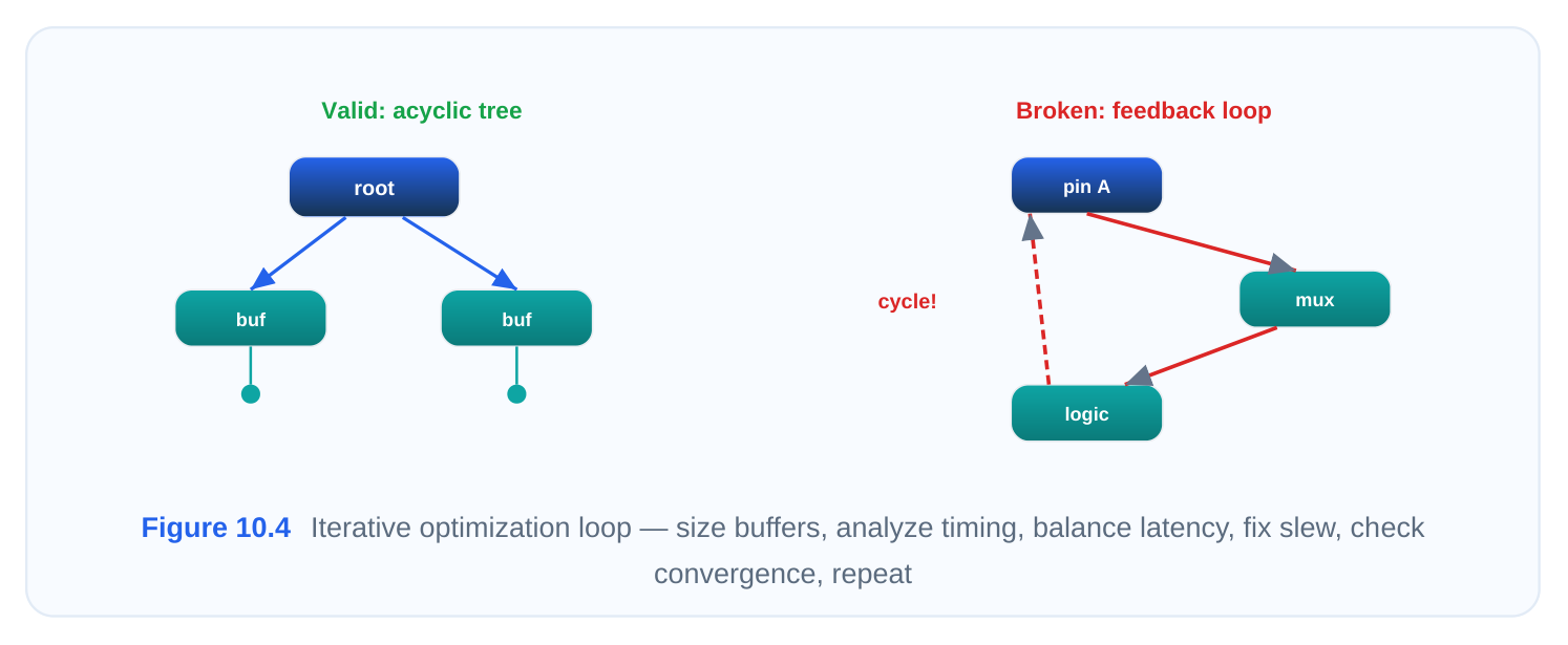
Phase 5 — Reporting
After optimization converges (or hits its effort/iteration ceiling), the tool finalizes the tree and emits a report bundle. This includes the achieved skew, minimum and maximum insertion delay (latency), worst clock-pin transition, buffer and inverter counts, total clock area added, and any constraints it could not meet. This phase is quick, but it is the most important one for you — it is the verdict on the run. Always read it before moving to clock routing and post-CTS optimization.
10.3 Runtime Expectations
One of the most common interview and on-the-job questions is simply: "How long should CTS take?" The honest answer is "it depends on the design," but you should carry calibrated expectations so you can recognize abnormal behavior. The figures below assume a single moderate block (tens of thou‐ sands of flops) on typical compute; they scale roughly with sink count, corner count, and effort.
| Scenario | Typical Runtime | What's Driving It |
|---|---|---|
| Small/clean block | 1–9 min | Few sinks, loose constraints, low congestion |
| Complex block | 9–28 min | Many sinks, multiple clocks, MMMC corners |
| Very congested block | 30+ min | Legalizer struggling for sites, routing hotspots |
| High-effort mode | 5–10× the base | Extra optimization passes for tighter skew/slew |
Several factors push you up these tiers. Sink count is the biggest lever — more flops means a bigger tree and more balancing work. Number of clocks and generated clocks multiplies the problem, es‐ pecially when they share registers. Corner and mode count under MMMC multiplies analysis cost on every optimization iteration. Constraint tightness matters enormously: a very aggressive skew or slew target forces the engine to keep iterating instead of declaring victory early. And congestion in the placement directly inflates the legalization phase.
The high-effort multiplier deserves special attention. When you crank optimization effort to its highest setting, you are telling the tool to run more refinement passes and search a larger solution space. It is realistic for a high-effort run to take five to ten times as long as the same design at nominal effort. That cost can be worth it for a final, sign-off-quality tree, but it is wasteful during early iterations when you are still shaking out constraint bugs.
10.4 Progress Monitoring
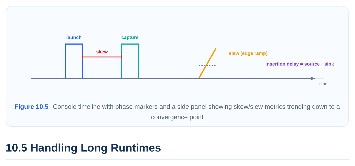
CTS is not a black box while it runs. The tool streams progress to the console (and the log file), and learning to read that stream is how you catch problems early instead of waiting twenty minutes for a bad result. Console messages. As the engine moves through the phases, it prints milestone messages: how many clocks it found, how many sinks per clock, which topology it chose, when it begins legalization, and when it enters optimization. Watch the sink counts first — they confirm the tool is building the tree you intended. A clock that reports zero sinks usually means a broken constraint; a clock reporting way too many sinks often means a missing exception that let the clock bleed into data logic. Status and iteration indicators. During the optimization phase the tool typically prints per-iteration status: current worst skew, current worst transition, number of buffers inserted so far, and the like. If you see these numbers improving iteration over iteration and then flattening, the engine is converging normally. If they oscillate or refuse to improve, the tool is fighting an over-constrained target. Completion and convergence metrics. At the end, the summary reports the final achieved values against your targets. The key ones to scan:
# After the run, pull the verdict numbers
report_clock_tree            ;# structure, levels, buffer/inverter counts
report_clock_timing -skew    ;# achieved skew vs target
report_clock_timing -latency ;# min/max insertion delay
report_clock_timing -transition_time  ;# worst clock-pin slew
report_constraint -all_violators       ;# anything CTS could not satisfy
The word "convergence" is worth pinning down for an interview. CTS converges when successive op‐ timization iterations stop producing meaningful improvement in the metrics it is chasing. A good con‐ vergence means it stopped because it met the targets. A bad convergence — sometimes called pre‐ mature termination — means it stopped because it hit an iteration or effort limit while still violating, and it simply gave up. The reports tell you which case you are in: meeting targets versus a non-empty violator list.
When a run is dragging on far past your expectation — or worse, finishing slow and with violations — you have several levers. Pull them in roughly this order, from least to most invasive. Loosen constraints first. The single most common cause of an endless optimization phase is a skew or transition target that is tighter than the design physically needs. If you asked for 27 ps of skew but your downstream timing only requires 72 ps, the tool burns enormous effort chasing precision that buys you nothing. Relax the target to what timing actually demands and the optimization phase often shrinks dramatically. The same applies to overly aggressive max-transition or max-capacitance rules.
# Trade unnecessary precision for runtime
set_clock_tree_options -target_skew 72   ;# was an over-tight 30
set_clock_tree_options -max_transition 225
synthesize_clock_trees
Choose the right algorithm and effort. Do not run high-effort mode on early, throwaway iterations. Use nominal or low effort while you are still validating constraints and exceptions, and reserve high effort for the run you intend to keep. Similarly, if your tool offers a choice of topology engine, picking the clustered/custom engine over a forced H-tree on an irregular design avoids wasted work. Scoping the run to a single clock or a subset of corners while debugging also slashes turnaround. Prepare the placement. CTS quality and speed both depend heavily on what it inherits. A cleanly legalized, not-overly-dense placement with congestion already under control lets the legalization phase find buffer sites quickly. If placement is congested, the legalizer thrashes. Fixing congestion be‐ fore CTS — through better placement, density screens, or relieving hotspots — is often the highestleverage runtime fix even though it happens upstream of the command. Improve legalization conditions. If buffers are struggling to land legally, give them room: reserve area for clock buffering in dense regions, check that placement blockages and keep-outs are not boxing the tree into a corner, and confirm your buffer cell list includes a healthy range of sizes so the engine has flexibility. A tree that has only one buffer size available will insert far more cells and spend longer legalizing them.
Finally, treat a slow run as diagnostic information. A run that is slow because it is converging well on a genuinely large design is fine — that is the cost of the work. A run that is slow because it is oscillating against an impossible target is telling you to change the inputs, not to wait longer. Reading the console mid-run (Section 10.4) is what lets you tell those two situations apart before you have wasted half an hour.
Interview Q&A
error-prone? It takes no required arguments because all the information it needs is already captured in the design's configuration state — the clock definitions, the CTS specification (skew, latency, slew, capacitance targets), the allowed buffer/inverter list, the NDRs, and the current placement. The command is a trigger that consumes that accumulated state. It is not especially error-prone because of the empty syntax; the errors come from misconfigured inputs, which you catch by reading the early console messages (sink counts) and the final reports. The design philosophy is "configure thoroughly once, then execute simply."
There are five: endpoint identification (trace from roots to find all sinks), topology creation (decide Htree versus clustered structure), legalization (place buffers on legal, non-overlapping sites while avoiding congestion), timing optimization (size buffers, balance insertion delay, minimize skew, fix slew and capacitance), and reporting. Timing optimization is by far the most expensive because it is iterative — it loops sizing, analysis, and balancing across all corners and modes until it converges or hits its effort ceiling, which is why it can run from a minute to many minutes.
and what do you check? I'd first ask how big the block is, how many clocks and corners are involved, and what effort level they used — 45 minutes can be perfectly normal for a large, multi-corner, high-effort run. Then I'd look at the live console: are the skew and slew metrics still improving iteration over iteration, or oscillating? Improving means it is genuinely converging and the time is justified. Oscillating means it is fighting an over-tight target. I'd also check the congestion of the input placement, since a thrashing legalizer is a classic time sink. The fix is usually to loosen an unnecessarily aggressive skew/transition target, drop effort on debug iterations, or relieve placement congestion upstream.
Convergence just means successive iterations stopped improving — it does not by itself mean success. Good convergence is when the engine stopped because it met the targets: the reports show achieved skew, latency, and transition within spec and an empty violator list. A bad outcome is premature termination, where the engine stopped because it hit an iteration or effort limit while still violating. Both "finish," but only one is acceptable. You tell them apart by reading the end-of-run
reports — report_constraint -all_violators and the clock-timing reports — not by the fact that the command returned.
Key Takeaways
synthesize_clock_treesneeds no required arguments because it derives every parameter from the design's prior configuration — clock definitions, the CTS spec, the buffer list, NDRs, and place‐ ment.- The run proceeds through five phases: endpoint identification, topology creation (H-tree vs. clustered), legalization, timing optimization, and reporting — with timing optimization the longest and most iterative.
- Calibrate your expectations: roughly 1–9 minutes for clean blocks, 10–30 for complex ones, 30+ when congested, and 5–10× when running high effort.
- Monitor the console live: confirm sink counts early, and watch skew/slew metrics trend toward convergence so you can catch over-constrained or premature-termination runs.
- When runtimes balloon, loosen unnecessarily tight constraints first, then tune effort and topology choice, then attack placement congestion and legalization conditions upstream.
- A slow run is diagnostic: slow-but-converging is the cost of real work, while slow-and-oscillating means the inputs, not the patience, need to change.
Comments
Leave a Reply