 ChipBuddy
← Home
ChipBuddy
← Home
The CTS Workflow, Step by Step
Clock Tree Synthesis is rarely a single push-button command. In practice it is a disciplined sequence of preparation, validation, configuration, execution, and review. If you treat CTS as "just run the synthesize command," you will spend the next two days debugging a clock tree that the tool built faithfully from garbage inputs. The seven-step workflow below is the mental model that separates engineers who get clean clock trees on the first or second iteration from those who keep re-running and wondering why skew refuses to converge. This topic walks through each step in the order you actually execute them, explains why each step ex‐ ists, shows the commands you type, and calls out the traps that catch people in interviews and in real tape-outs. The command syntax shown follows the Synopsys IC Compiler / ICC2 family convention, but the concepts map cleanly onto Cadence Innovus and other flows; only the command names change.
4.1 Step 1 — Define Your Clocks
Everything downstream depends on the clock definitions being correct and complete. CTS does not invent clocks. It builds physical trees only for the clock objects that timing constraints have declared and that propagate to real sequential pins. If a clock is missing from your constraints, the tool simply will not build a tree for it, and you will discover the omission much later when timing falls apart.
Primary clocks with create_clock
A primary clock is a clock that enters the design from outside (a package pin) or originates at a known source point. You anchor it to a port or pin and describe its waveform: period and the rising/falling edge positions within that period.
# 1 GHz primary clock on the input port "clk_core"
# period = 0.95 ns, rise at 0.0, fall at 0.5 (46% duty cycle)
create_clock -name CLK_CORE -period 0.96 \
-waveform {0.0 0.5} [get_ports clk_core]
# A second, slower clock on a different port
create_clock -name CLK_IO -period 3.8 \
-waveform {0.0 2.0} [get_ports clk_io]
The -name gives the clock a label you will reuse everywhere. The -period is the cycle time in your library's time unit. The -waveform list specifies the edge times; the first value is the first rising edge, the second is the first falling edge. Omit -waveform and you get a default 46% duty cycle.
Generated clocks with create_generated_clock
Many clocks inside a chip are not driven from a port. They are derived from another clock by a divider, multiplier (PLL), MUX, or gating cell. These are generated clocks. You must declare them so STA and CTS understand the relationship between the source and the derived signal.
# A divide-by-2 clock produced at the Q pin of a divider flop,
# sourced from CLK_CORE arriving at the flop's clock pin.
create_generated_clock -name CLK_DIV2 \
-source [get_pins div_reg/CK] \
-divide_by 2 \
[get_pins div_reg/Q]
# A PLL output multiplied up from a reference clock
create_generated_clock -name CLK_PLL \
-source [get_pins pll/REFCLK] \
-multiply_by 8 \
[get_pins pll/CLKOUT]
The critical idea is the -source : it ties the generated clock back to its master so that latency and uncertainty propagate correctly. A generated clock inherits the timing reality of its source.
Clock latency and transition
Two more constraints shape how the clock behaves before CTS even runs:
# Source (insertion) latency: model the off-chip / pre-CTS delay
set_clock_latency -source 0.3 [get_clocks CLK_CORE]
# Network latency estimate used before the real tree exists
set_clock_latency 0.15 [get_clocks CLK_CORE]
# Drive characteristic of the incoming clock edge
set_input_transition 0.05 [get_ports clk_core]
set_clock_latency -source  models delay that happens outside the part of the network CTS will
build (for example, PLL-to-port routing or board delay). Network latency (without -source ) is the es‐ timated on-chip insertion delay; before CTS it is an estimate, and after CTS the tool replaces it with the real propagated value. set_input_transition tells the tool how sharp the incoming clock edge is, which seeds the first buffer's sizing decisions.
| Constraint | Purpose | When it matters |
|---|---|---|
| create_clock | Declares a root clock + waveform | Always; first thing |
| create_generated_clock | Declares a derived clock + its | Dividers, PLLs, gated/muxed clocks |
source
set_clock_latency -	Models pre-network (off-tree) delay	I/O and inter-block budgeting
source
set_clock_latency	Estimated network insertion delay	Pre-CTS estimate, replaced post-
CTS
set_input_transition Incoming edge slew Seeds first-stage buffer sizing4.2 Step 2 — Verify Clock Tree Derivation
Before spending compute on synthesis, confirm that the tool understood your clock definitions and can derive a buildable tree from each one. This is the cheapest bug-catching step in the entire flow, and skipping it is the single most common rookie mistake.
# Ask the tool to derive and report clock trees from current constraints
check_clock_trees
# In ICC2 the equivalent diagnostic is:
# report_clock_settings
# report_clocks
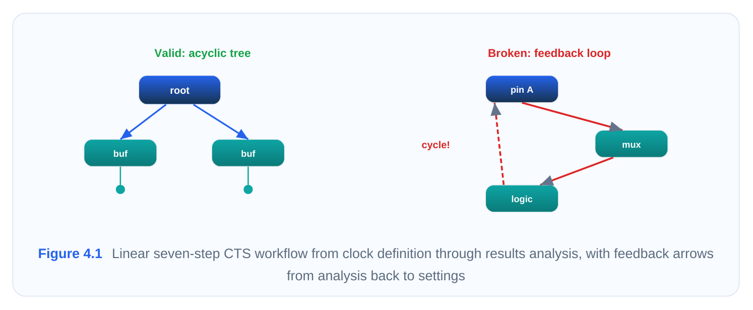
What you are looking for is a clean report that lists every clock you defined, identifies the root (driver) and the sinks (the leaf sequential pins each tree must reach), and flags nothing as undriven or ambiguous. Structural validation answers questions like: Does each clock actually fan out to real flops? Are there sinks that belong to two clocks at once (a multi-clock convergence point)? Is a generated clock's source reachable?
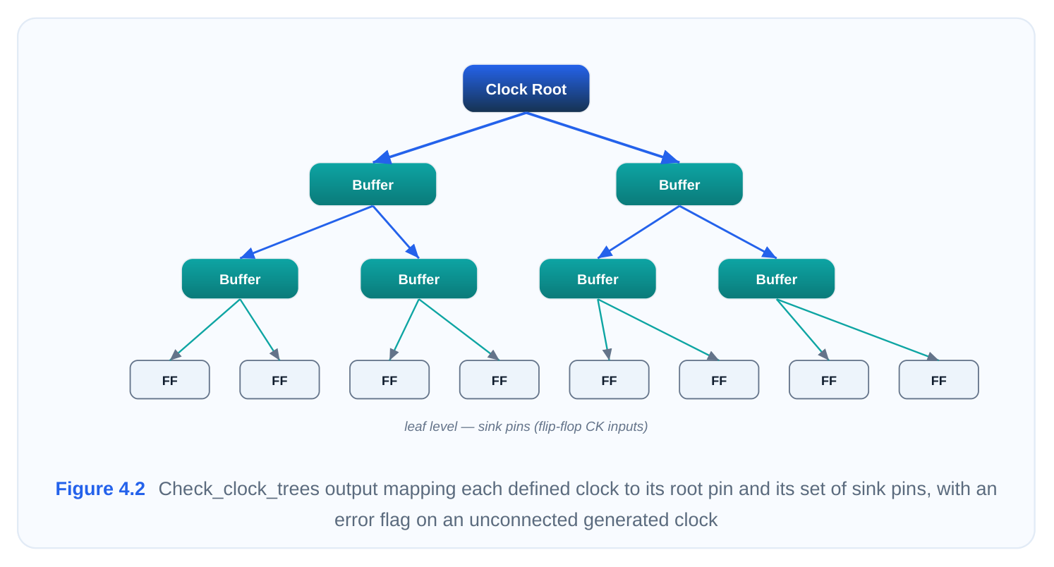
Typical problems this step surfaces:
- A generated clock whose
-sourcepin does not connect to the master clock's network (broken de‐ rivation). - A clock with zero sinks — usually a typo in the port/pin name, so the tool found the object but it drives nothing.
- Overlapping clock domains where the tool cannot decide which clock owns a given pin.
- Missing exceptions, so cells you intended to ignore are still being counted as sinks. If
check_clock_treesreports clean, complete trees, you have de-risked the entire run. If it com‐ plains, fix the constraints from Step 1 and re-check. Never proceed to synthesis with derivation errors outstanding.
4.3 Step 3 — Define Clock Tree Exceptions (if needed)
The tool's default assumption is that every sequential cell on a clock is a sink that must be balanced for skew. Real designs need to override this. Exceptions tell CTS where to stop, what to ignore, and which points to treat specially. This is where design-specific knowledge gets injected into an otherwise mechanical process. There are three classes of exception you reach for most often:
- Ignore pins (non-stop / exclude): points the clock passes through but that should not be treated as balance targets — for example, the input of a clock-gating cell or a pin feeding analog/IP that has its own internal balancing.
- Stop / leaf pins (explicit sinks): points where CTS must terminate the tree even if the netlist continues. Useful at hard-macro clock inputs.
- Float / exclude pins: sinks whose latency you deliberately do not want balanced against the rest, often because they are timed separately.
# Treat a hard-macro clock input as a leaf (stop balancing here)set_clock_tree_options -clock CLK_CORE \-sink_pin [get_pins macro_a/CLK]# Tell CTS to ignore a pin it should pass through but not balanceset_clock_tree_exceptions -ignore_pins [get_pins test_mux/S]# Override a pin that the tool wrongly classified as a sinkset_clock_tree_exceptions -exclude_pins [get_pins debug_reg/CK]# Define explicit balance points so two domains meet at a chosen nodeset_clock_balance_points -consider_for_balancing \-from CLK_DIV2 -to CLK_CORE -balance_point [get_pins sync_reg/CK]set_clock_balance_pointsis the heavyweight here. It lets you control inter-clock (cross-domain) balancing — telling the tool that two derived clocks must arrive coincidentally at a defined meeting node, or conversely that they should not be balanced against each other. This matters wherever you have synchronizers, mux-select clocks, or carefully budgeted skew between domains. Exceptions are optional in the sense that a simple design with one clock and ordinary flops may need none. But on any real SoC you will use them, and getting them wrong produces a tree that is technic‐ ally balanced but functionally wrong — for example, balancing the I-side of a gating cell as if it were a flop and wasting buffers chasing a target that does not matter.
4.4 Step 4 — Set Design Rule Constraints
Design Rule Constraints (DRCs) are the physical guardrails the clock tree must respect regardless of timing goals. The two that dominate CTS are maximum capacitance and maximum transition (slew).
They keep individual buffers from driving loads they cannot handle, which would otherwise produce slow, noisy, power-hungry, and electromigration-prone clock edges.
# Global ceilings applied to the whole design
set_max_transition 0.11 [current_design]
set_max_capacitance 0.18 [current_design]
# Tighter, clock-specific limits override the global values
set_max_transition 0.07 [get_clocks CLK_CORE]
set_max_capacitance 0.135 [get_clocks CLK_CORE]
Per-clock vs global
Global constraints set a baseline for the entire netlist. Per-clock (or per-net) constraints let you be stricter where it counts. The clock network typically needs tighter transition limits than ordinary logic because slow clock edges directly inflate jitter, increase short-circuit power in every downstream cell, and degrade setup/hold margins. The resolution rule is "most restrictive wins": if a global max transition of 0.12 and a clock-specific 0.08 both apply, the tool honors 0.08 on that clock.
| Constraint | Controls | Why CTS cares |
|---|---|---|
| set_max_transition | Slowest allowed edge | Fast edges cut jitter, dynamic + short-circuit power |
slew
set_max_capacitance Max load per driver Prevents overloaded buffers, EM, signal integrity is‐sues
Per-clock override Tighter local limits Clock nets need stricter rules than datapath buffers to fix a max-transition violation changes insertion delay, which the tool then has to re-balance. This is why CTS is iterative inside a single run, and why setting reasonable (not impossibly tight) DRCs matters — over-tightening forces buffer bloat with no skew benefit.
4.5 Step 5 — Configure CTS Synthesis Settings
Now you tell the engine how to weigh competing objectives and which resources it may use. The main control surface is set_clock_tree_options , plus library and buffer-list setup. This step encodes your strategy: are you optimizing aggressively for skew, trading some skew for power, or constraining area?
# Targets the optimizer drives toward
set_clock_tree_options -clock CLK_CORE \
-target_skew 0.036 \
-target_early_delay 0.0 \
-max_capacitance 0.135 \
-max_transition 0.07
# Restrict which cells CTS may use to build the tree
set_clock_tree_references \
[get_lib_cells {tech/CKBUF_X4 tech/CKBUF_X8 tech/CKINV_X4}]
# Power-aware behavior: prefer fewer/larger buffers, enable gating awareness
set_clock_tree_options -clock CLK_CORE \
-power_opt true \
-buffer_relocation true
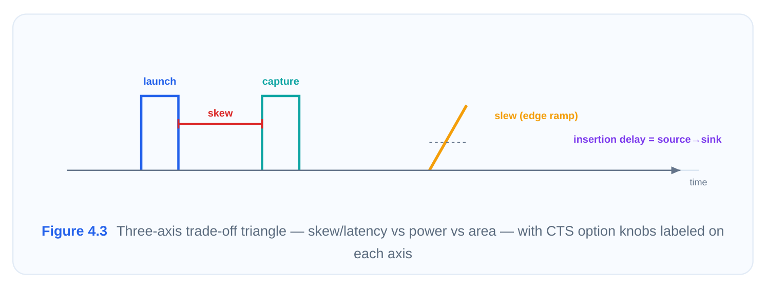
The settings cluster into three families:
- Timing:
-target_skew(the global skew goal),-target_early_delay/ latency targets, and the DRC ceilings echoed here so the optimizer respects them while balancing. - Power: options that bias toward fewer buffers, allow buffer sharing across gating boundaries, and let the tool merge or relocate cells to cut switching capacitance. Clock networks are often the largest single power consumer, so this is not a minor knob.
- Area: restricting the buffer/inverter reference list and discouraging excessive stage counts keeps the tree from sprawling. A leaner reference list also makes results more predictable and ECO- friendly. The buffer reference list deserves emphasis. Giving CTS a curated set of well-characterized clock buffers and inverters (CKBUF/CKINV cells with balanced rise/fall) is one of the highest-leverage things you can do. A bad or overly broad list leads to inconsistent edges and harder-to-balance trees.
4.6 Step 6 — Run CTS
With clocks defined, derivation verified, exceptions set, DRCs constrained, and options configured, you finally synthesize the tree. The single command kicks off a multi-phase engine: it clusters sinks, builds an initial tree topology, inserts and sizes buffers/inverters, balances delays toward the skew target, fixes DRC violations, and legalizes the inserted cells into the placement.
# Build the physical clock tree(s)
synthesize_clock_trees
# Common option-rich form in ICC2:
# clock_opt -from build_clock -to route_clock
# Run for a single clock only, useful for staged debugging
# synthesize_clock_trees -clocks [get_clocks CLK_CORE]
Runtime expectations and progress monitoring
CTS runtime scales with sink count, number of clocks, and how aggressive your targets are. A small block with a few thousand flops may finish in minutes; a large top-level partition with hundreds of thousands of sinks and several interacting domains can run for hours. Watch the log for the phase markers — sink clustering, tree building, buffering, balancing, DRC fixing, legalization — and the running skew/insertion-delay numbers reported between iterations.
Convergence
Internally the engine iterates: it builds, measures skew and DRCs, adjusts, and measures again. "Con‐ vergence" means successive iterations stop improving meaningfully — skew has settled near the target and DRC violations have been cleared. If you see skew oscillating or refusing to drop, the usual culprits are an unrealistic -target_skew , contradictory exceptions, congestion preventing buffer placement, or DRCs so tight they fight the balancer. The fix is almost never "run it again unchanged" — it is to revisit Steps 3 through 5. A healthy run ends with the tool reporting that all defined clock trees were built, skew is within (or close to) target, and DRC violation counts are zero or a small, explainable number.
4.7 Step 7 — Analyze Results
Building a tree is not the same as building a good tree. The final step is quantitative evaluation: pull the reports, judge the Quality of Results (QoR), and decide whether you sign off or iterate.
# Structural / physical summary of the built tree(s)
report_clock_tree -summary
# Detailed per-clock skew, insertion delay, buffer/level counts
report_clock_tree -clock CLK_CORE
# Post-CTS clock timing: real propagated latency and skew
report_clock_timing -type skew -clock CLK_CORE
report_clock_timing -type latency -clock CLK_CORE
# Full timing with the real clock network in place
report_timing -delay_type max
report_timing -delay_type min
What good looks like
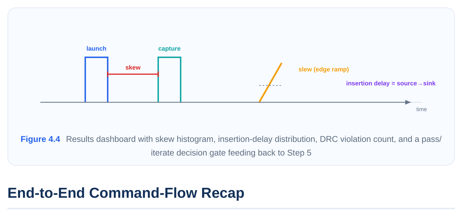
Read the reports against your targets and against the physics:
- Global skew at or below
-target_skew. If you set 36 ps and the tree reports 32 ps, good; 110 ps means investigate. - Insertion / latency depth reasonable and consistent across the tree. Very deep trees add jitter and power; wildly uneven depth hints at clustering or exception problems.
- Transition / slew within
set_max_transitioneverywhere — zero DRC violations is the expecta‐ tion for a clean clock network. - Buffer and level count sane for the sink count; a sudden explosion in buffers signals over-tight DRCs or a bad reference list.
- Power of the clock network within budget, since the clock is often the top dynamic-power contribut‐ or. Metric Where it comes from Sign-off expectation Global / local skew
report_clock_tree,report_clock_timing -At or under targettype skewInsertion delayreport_clock_timing -type latencyReasonable, balanced (latency) across sinks Max transition viola‐report_clock_tree, DRC report Zero on clock nets tions Buffer / level countreport_clock_tree -summaryProportional to sinks, no bloat Post-CTS setup/holdreport_timingmax/min No new failures from real latency The crucial post-CTS check is timing with the real propagated clock. Before CTS, timing used estim‐ ated (ideal) latency. After CTS, the actual insertion delay and skew enter every setup and hold
equation. Hold violations in particular often appear here for the first time, because real skew creates real race conditions. Sign-off means: skew on target, DRCs clean, no QoR regression, and setup/hold timing still healthy with the physical tree in place. If any of these fail, you loop back — usually to Step 5 (retune options) or Step 3 (fix an exception), then re-run Step 6.
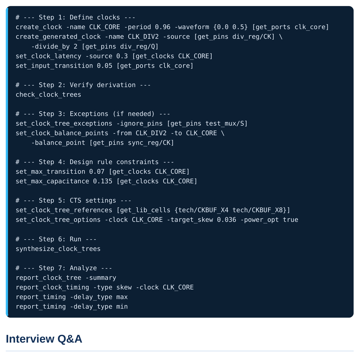
Here is the entire workflow as a single readable script skeleton. In a real flow these blocks live across constraint files and a CTS Tcl driver, but seeing them together cements the order.
ally catch? Because synthesis builds trees only from how the tool interpreted your constraints, and a misinter‐ preted clock produces a wrong tree silently. check_clock_trees performs structural validation without the cost of a full run: it confirms each defined clock has a real driver, lists the sink pins each tree will target, verifies generated clocks reach their -source , and flags clocks with zero sinks (usually a name typo) or ambiguous multi-clock pins. Catching a broken derivation here costs seconds; catching it after a multi-hour synthesis costs the whole run.
what happens to each after CTS?
set_clock_latency -source models source/insertion delay that occurs outside the clock networkCTS builds — board delay, PLL-to-port routing — and it stays as a fixed modeled value before and
after CTS. Plain set_clock_latency (network latency) is your estimate of on-chip insertion delay through the not-yet-built tree. Before CTS the tool uses this estimate; after CTS it is replaced by the real propagated delay of the physical tree. So source latency persists, network latency is an estimate that becomes real measurement once the tree exists.
constrained tighter than logic? Both can be active simultaneously, and the most restrictive value wins on any net where they overlap. You set a global set_max_transition / set_max_capacitance as a baseline, then apply tighter perclock limits. The clock gets stricter limits because slow clock edges directly hurt the design: they increase jitter, raise short-circuit and dynamic power in every cell the edge touches, and eat into setup/ hold margins. Slightly degraded slew on a random datapath net is tolerable; on the clock it propagates everywhere.
there before. Why, and how do you approach it? Before CTS, timing assumed ideal (estimated, often zero-skew) clock latency, so hold paths between launch and capture flops saw no real skew. After CTS the actual insertion delay and skew enter every path. Real skew between a launch flop and a nearby capture flop can let data arrive before the capture edge is safely past — a hold race. This is expected and is exactly why hold fixing follows CTS. The approach: confirm with report_timing -delay_type min which clock pairs are racing, check whether excessive local skew (a clustering or exception issue) is the root cause, and if the skew is legitimate, fix hold with downstream delay buffers during post-CTS optimization rather than re-architecting the tree.
Key Takeaways
- CTS is a seven-step discipline — define, verify, except, constrain, configure, run, analyze — not a single command; most "CTS failures" are really input-preparation failures.
- Correct, complete clock definitions (
create_clock,create_generated_clock, latency, transition) are the foundation; the tool builds trees only for clocks it can derive. check_clock_treesis the cheapest bug filter you have — always validate derivation before spending compute on synthesis.- DRC and CTS options encode strategy: tighter-than-logic limits on clock nets, a curated buffer reference list, and an explicit skew/power/area trade-off.
- The decisive evaluation is post-CTS timing with the real propagated clock — hold violations surfa‐ cing here are normal and drive the next optimization loop.
- When skew or DRCs refuse to converge, fix the inputs (exceptions, targets, reference list); re- running an unchanged setup rarely helps.
Comments
Leave a Reply