 ChipBuddy
← Home
ChipBuddy
← Home
Post-CTS Analysis & Reporting
Once the clock tree has been built and the design has been legalized after CTS, the real work of judging whether the tree is any good begins. Building buffers and routing the clock nets is only half the story. The other half is proving, with hard numbers, that the tree meets your latency targets, that skew is under control across every clock domain, that the cells you dropped in did not break placement legality, that the extra clock routing did not choke the channels reserved for signal nets, and that the clock network is not silently blowing through your power budget. This is the post-CTS analysis and reporting stage, and it is where an experienced physical-design engineer earns their keep. This topic walks through the commands and the mental models you need to interrogate a clock tree after synthesis. We will cover the two workhorse reporting commands ( report_clock_tree and re‐ port_clock_timing ), then move into design-rule validation, congestion inspection, and clock-power assessment. The exact switch names below follow the Synopsys IC Compiler II / Fusion Compiler family conventions, but the concepts map cleanly onto Cadence Innovus and other tools — only the syntax differs.
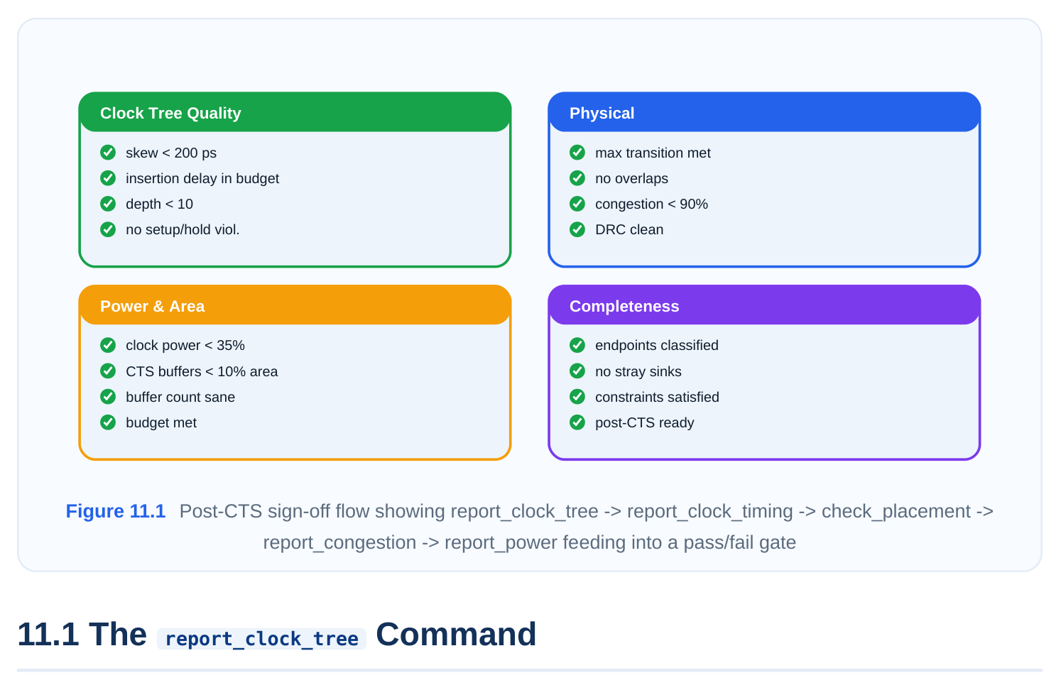
report_clock_tree is your structural and electrical summary of the synthesized tree. Think of it asthe "what did CTS actually build" report. It answers questions about how deep the tree is, how many buffers and inverters were inserted, how much capacitance is hanging off the network, and how much power that network is expected to burn. It is the first command most engineers run the instant CTS finishes, because it gives a fast sanity read before you spend time on detailed timing.
11.1.1 The -summary View: Depth, Buffers, Capacitance, Power
The -summary switch collapses the entire tree into a compact table per clock. It is meant for a quick glance, not a deep dive. The fields you care about are the tree depth (the number of buffer stages from the clock source to the leaf flops), the total count of clock buffers and inverters inserted, the aggregate capacitance driven by the network, and an estimate of the clock-network power.
# Quick structural + electrical summary of every clock tree
report_clock_tree -summary
# Restrict the summary to a single clock
report_clock_tree -summary -clock [get_clocks CLK_CORE]
A typical summary table looks like this:
| Clock | Levels (depth) | Buffers | Inverters | Sinks | Total Cap (pF) | Net Power (mW) |
|---|---|---|---|---|---|---|
| CLK_CORE | 7 | 412 | 38 | 9,840 | 184.2 | 22.6 |
| CLK_DDR | 5 | 96 | 12 | 1,210 | 41.7 | 6.1 |
| CLK_PERI | 6 | 58 | 0 | 640 | 19.3 | 2.4 |
How do you read this? Depth tells you about balance and latency risk. A very deep tree (say, more than 7–9 levels on a normal block) usually signals that the tool struggled to balance loads, or that your max_fanout or max_capacitance constraints forced it to stack stages. Depth directly inflates insertion delay and makes the tree more sensitive to on-chip variation (OCV), because every extra stage adds a launch/capture path segment that can be derated differently. Buffer and inverter counts feed straight into area and, more importantly, power. If CLK_CORE above is burning 22.6 mW just to distribute the clock, that is a number your power lead will want to see early.
11.1.2 Detailed QoR Metrics: Per-Clock Insertion Delay and Skew
When you drop -summary and ask for the full QoR (Quality of Results) report, the tool expands into per-clock detail. Now you get insertion delay (also called clock latency — the propagation time from the clock definition point to the leaf pins), and you get skew broken out as the spread between the earliest-arriving and latest-arriving sinks.
# Full per-clock QoR with latency and skew breakdown
report_clock_tree -qor
# Same, but only the core clock, with verbose stage detail
report_clock_tree -qor -clock [get_clocks CLK_CORE] -verbose
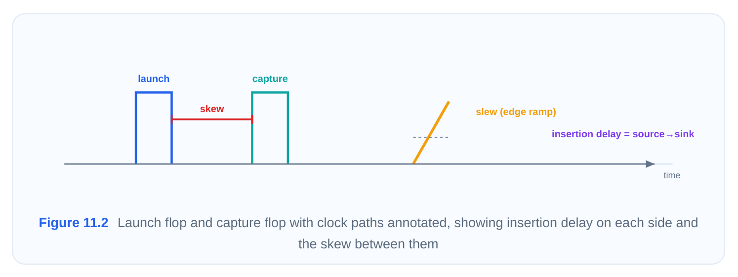
The distinction that trips up junior engineers in interviews is the difference between global skew and local skew. Global skew is the difference between the longest and shortest insertion delay across all sinks of a clock. Local skew is the difference only between sinks that are actually in a timing relationship with each other (i.e., a launch flop and the capture flop it talks to). Local skew is what genuinely matters for setup and hold; global skew is an easier-to-compute proxy. A tree can have ugly global skew but perfectly acceptable local skew if the far-apart flops never communicate.
| Metric | What it measures | Why it matters |
|---|---|---|
| Insertion | Source-to-sink clock propagation delay | Higher latency = more OCV exposure, harder hold |
| Global skew | Max minus min latency across all sinks | Coarse balance indicator |
| Local skew | Skew between related launch/capture | Directly drives setup/hold margin |
pairs
| Max transition | Worst slew on any clock pin | DRV health; affects power and duty cycle |
|---|---|---|
| Latency range | Min/max latency window per clock | Used to budget useful skew |
11.1.3 The -format table Option: Spreadsheet-Friendly Output
For documentation, regression dashboards, or just dumping into a spreadsheet, the tabular format is invaluable. Instead of the free-flowing text block that the default report produces, -format table emits clean, column-aligned rows that you can redirect to a file and parse with awk , import into Excel, or feed into a CI dashboard.
# Emit a tabular, machine-parseable QoR report and save it
report_clock_tree -qor -format table > ./reports/cts_qor.rpt
# Many flows let you constrain which columns appear
report_clock_tree -qor -format table \
-columns {clock levels buffers max_latency min_latency global_skew} \
> ./reports/cts_qor_trimmed.rpt
The practical win here is reproducibility. When you run CTS twenty times across an optimization sweep, you want each run to produce an identically structured file so a diff or a trend plot is trivial. The default human-readable format breaks scripted parsing the moment the tool changes a word; the table format is far more stable. In a real flow you will typically wrap this in a Tcl redirect block so the re‐ port lands in a per-run directory keyed by the run timestamp.
11.1.4 Custom Filters and Options
The tree can be enormous, so filtering is essential. You rarely want every one of ten thousand sinks dumped to a log. The common filters let you target a specific clock, a specific corner or scenario, a depth threshold, or only the cells that violate a design rule. Useful options you should know cold:
-clock <list>— limit the report to named clocks rather than all clocks.-scenario/-corner— pick which analysis view the latency and power numbers come from (critical when you have multi-corner multi-mode setups).
-nosplit— prevent the tool from wrapping long instance names onto a second line, which keeps the output script-parseable.-significant_digits <n>— control numerical precision in the output.# Report only the worst offenders for the core clock in the slow cornerreport_clock_tree -qor \-clock [get_clocks CLK_CORE] \-scenario func_ss_125c \-nosplit -significant_digits 4The interview-level insight: always be explicit about which view your numbers come from. A clock tree that looks perfectly balanced in the typical corner can show meaningful skew in a slow, high-temperat‐ ure corner because cell delays and wire RC scale differently. If you report a single skew number without naming its corner, an experienced reviewer will immediately ask "which corner?" — and not having an answer is a red flag.
11.2 The report_clock_timing Command
Where report_clock_tree describes the structure, report_clock_timing is the analytical com‐ mand that quantifies the timing behavior of the tree. It is driven by a -type switch that selects what dimension you want to inspect: skew, latency, setup, or hold. This is the command you lean on when you need to defend the tree to a timing-closure lead.
11.2.1 -type skew : Min/Max Skew, Ranges, and Endpoint Skew
The skew report quantifies the arrival-time spread at the clock pins. With -type skew you get the minimum and maximum skew, the overall skew range per clock, and — when you ask for endpoint detail — the skew measured at specific register endpoints.
# Per-clock skew summary
report_clock_timing -type skew
# Skew with worst endpoint pairs called out
report_clock_timing -type skew -clock [get_clocks CLK_CORE] -nworst 10
When reading skew output, remember the sign convention. Positive skew (capture clock arrives later than launch) helps setup but hurts hold. Negative skew (capture arrives earlier) does the opposite. This is the basis of "useful skew," where you deliberately let the tool skew certain endpoints to borrow time across a tight path. So a non-zero skew number is not automatically bad — context decides whether it is helping or hurting.
| Skew condition | Setup effect | Hold effect | Typical CTS goal |
|---|---|---|---|
| Zero skew | Neutral | Neutral | Classic balanced tree |
| Positive (capture late) | Improves | Worsens | Borrow time on slow paths |
| Negative (capture early) | Worsens | Improves | Fix hold on fast paths |
11.2.2 -type latency : Source-to-Sink Insertion Delay
Latency mode reports insertion delay — the time it takes the clock edge to travel from its source to each leaf pin. You can get the latency from source to sink, and you can request per-endpoint latency to see exactly which flops sit at the extremes of the latency distribution.
# Insertion delay (clock latency) per clock
report_clock_timing -type latency
# Endpoint-level latency, sorted to find the deepest sinks
report_clock_timing -type latency -clock [get_clocks CLK_CORE] \
-nworst 20 -nosplit
Latency is the number that connects the tree to the rest of the timing world. High insertion delay is dangerous for two reasons. First, it increases your exposure to OCV: the longer the clock path, the more absolute uncertainty the derating factors inject, which eats into both setup and hold margins. Second, large source-to-sink latency widens the window in which clock-as-data and reconvergence effects matter. Many flows therefore set an explicit insertion-delay target during CTS and treat the post-CTS latency report as the proof that the target was hit.
11.2.3 -type setup : Setup Margins and Per-Clock Slack
With -type setup , the report folds the clock tree's contribution into setup analysis and shows you the setup margin — effectively the slack — on the clock-sensitive paths, broken out per clock.
# Setup margin contribution from the clock network, per clock
report_clock_timing -type setup -clock [get_clocks *] -nworst 5
This view matters because CTS changes setup behavior. Before CTS the tool worked with ideal clocks (zero latency, zero skew). After CTS the clocks are propagated, so real latency and real skew now factor into every setup check. A path that had comfortable setup slack under the ideal-clock assumption can tighten — or loosen — once propagated clocks are in play. The -type setup report is how you catch paths that CTS pushed into the danger zone, before you hand off to full static timing analysis.
11.2.4 -type hold : Hold Margins and Violation Detection
Hold is where CTS most often hurts you, so this is arguably the most important -type . After CTS, real skew and real latency expose hold violations that simply could not exist under ideal clocks. The hold report surfaces the hold margins and flags the endpoints that are failing.
# Hold margin and violation listing from the clock network
report_clock_timing -type hold -clock [get_clocks *] -nworst 20 \
> ./reports/cts_hold.rpt
The mechanism to understand: hold checks compare the launch and capture edges of the same clock cycle. When skew makes the capture clock arrive earlier than the launch clock (negative skew on that pair), the data can race through and arrive at the capture flop before its hold window closes. Long insertion delays amplify this because they spread the launch and capture paths physically apart, making them more vulnerable to mismatch and OCV derating. This is precisely why CTS is followed by a dedicated hold-fixing pass that inserts delay (buffers) on the data path — and the -type hold re‐ port is what tells you how much work that pass has ahead of it.
| -type value | Primary question answered | When you run it |
|---|---|---|
| skew | How balanced are the clock arrivals? | Immediately post-CTS |
CTS does not just route nets — it inserts physical cells (buffers and inverters) and legalizes them into rows. That cell insertion can introduce placement problems: cells placed on top of each other, cells violating minimum-spacing rules, or cells nudged outside the legal core or block boundary. Before you
trust any timing number, you must confirm the design is still physically legal. The command for this is
check_placement .
# Run the full battery of placement legality checks
check_placement -all
# Focus only on overlap and out-of-bounds issues, write a report
check_placement -verbose > ./reports/cts_placement_check.rpt
The -all switch runs every available check. The categories you most care about after CTS are:
- Overlap detection — two or more cells occupying the same site. After CTS this usually means newly inserted clock buffers were not properly legalized. Overlaps are hard errors; routing cannot proceed.
- Spacing violations — cells that are placed too close together to satisfy the technology's minimum- spacing or implant-layer rules. These are common around dense clock-buffer clusters.
- Out-of-bounds placement — a cell whose footprint extends past the core area, a hard macro keep-out, or a placement blockage. CTS can push buffers into forbidden regions when it is desperate for whitespace near a sink cluster.
- Row / orientation / site legality — cells not snapped to a legal row, or with an orientation the row does not allow. Check type What goes wrong post-CTS Typical fix Overlap Inserted buffers share sites Re-run legalization (
legalize_placement) Spacing Buffer clusters too dense Spread cells, add spacing margin Out-of-bounds Buffers pushed past core / into keep-out Reserve whitespace, re-place Row/site legality Cells off-grid or mis-oriented Legalize / snap to rows The discipline here is simple: a cleancheck_placement -allis a gate. If it does not pass, no down‐ stream report is meaningful, because routing will fail or the extracted parasitics will be garbage. Treat placement legality as a hard prerequisite, not a nice-to-have.
11.4 Congestion Analysis
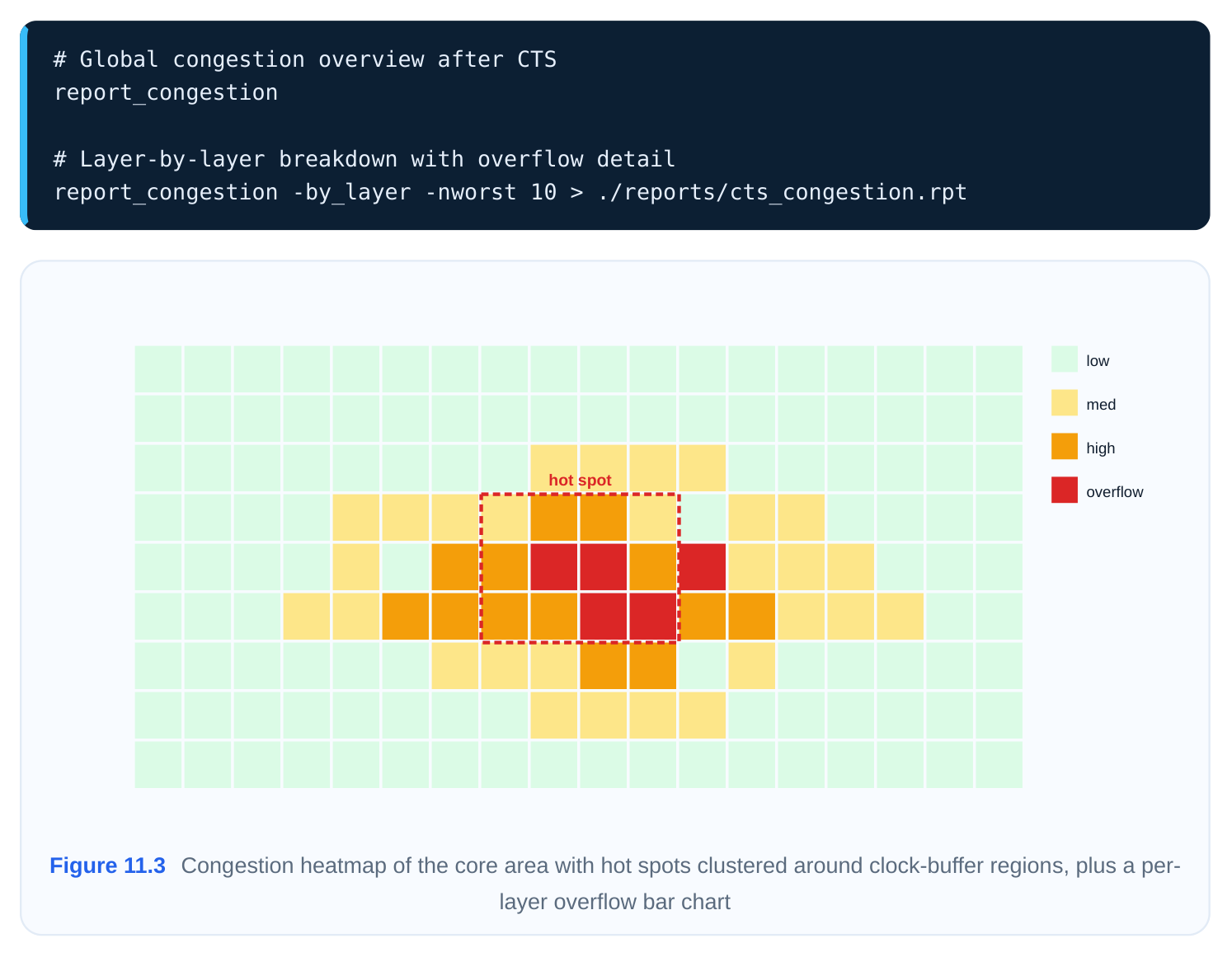
Every clock buffer and every clock net you add consumes routing resources. Clock nets are typically routed on higher metal layers with non-default rules (wider wires, extra spacing, sometimes shielding), which means they can eat disproportionately into the tracks available for signal routing. After CTS you must verify that the clock network has not created congestion hot spots that will make the design unroutable. The command is report_congestion .
Reading the Numbers
Congestion is reported as overflow: the demand for routing tracks in a given region (a global-routing cell, or GRcell) minus the supply of tracks available. Positive overflow means more nets want to cross that region than there are tracks to carry them. The report gives you both global statistics (total overflow, percentage of GRcells with overflow) and, with -by_layer , a per-metal-layer view. The layer-by-layer view is the one that matters most for CTS. Because clock routing tends to live on specific layers, you will often see overflow concentrate on exactly those layers. If your clock spine sits on, say, M5 and M6, watch for overflow spikes there.
| Layer | Tracks supplied | Tracks demanded | Overflow | Note |
|---|---|---|---|---|
| M2 | 12,400 | 9,800 | 0 | Healthy |
| M5 | 8,200 | 8,950 | +750 | Clock spine pressure |
| M6 | 7,900 | 8,610 | +710 | Clock spine pressure |
| M7 | 5,100 | 3,200 | 0 | Headroom |
Post-CTS vs. Baseline
The single most useful thing you can do is compare the post-CTS congestion picture against the preCTS (post-placement) baseline. The delta attributable to CTS is what you want to isolate. If overflow jumped by a meaningful margin on the clock layers after CTS, that increase is the price the clock tree charged you, and it tells you whether the design is still routable. If congestion is borderline, the levers are: reduce clock-buffer density, relax non-default routing rules where skew budget allows, move the clock spine to a less-contested layer, or add routing blockages to steer the buffers apart. The goal of this analysis is a confident "yes, this will route" before you commit to detailed routing.
11.5 Power Analysis
The clock network is almost always the single largest dynamic-power consumer in a synchronous design. Every clock buffer switches on every cycle, every clock net charges and discharges its capacit‐ ance twice per cycle, and the clock has the highest activity factor of any net in the design (it toggles at the clock frequency itself). After CTS you have, for the first time, a real clock network to measure — so this is when you validate the design against its power budget.
# Overall power, with the clock network broken out
report_power
# Isolate the clock-network power contribution
report_power -clock_network > ./reports/cts_clock_power.rpt
Decomposing Clock-Network Power
Power splits into two big buckets: dynamic and leakage (static).
- Dynamic power has two sub-components. Switching power is the energy spent charging and dis‐ charging the net capacitance (proportional to C · V² · f · activity). Internal power is the short-circuit and internal-cap power burned inside the buffer cells when they switch. For the clock network, dynamic power dominates because the activity factor is effectively 1 — the clock never idles.
- Leakage power is the static current that flows through the clock buffers even when they are not switching. With hundreds or thousands of always-on clock buffers, leakage adds up, especially in hot corners and with low-Vt cells. CTS cell selection (high-Vt vs. low-Vt buffers) is a direct lever on leakage. Power component Source in the clock tree Main lever Switching Charging/discharging net capacitance Net length, wire width, buffer count Internal Short-circuit + internal cap in buffers Buffer sizing, slew control Leakage Static current through always-on buffers Vt flavor selection
Validating Against the Budget
The post-CTS power number is checked against the clock-power portion of the project's power budget. If report_power -clock_network shows the tree exceeding its allocation, you have several optimiza‐ tion paths: enable or improve clock gating so portions of the tree go quiet when idle (this attacks the activity factor, the biggest dynamic-power driver); choose higher-Vt buffers to cut leakage; reduce buffer count and tree depth where the latency budget allows; and tighten capacitance by shortening clock routes. Clock gating is usually the highest-impact move because it directly reduces the effective activity of large swaths of the tree. The interview-worthy summary: clock power is dominated by dynamic switching because of the clock's unity activity factor, the network's large total capacitance, and its high buffer count. Reducing it is mostly about gating the clock off where it is not needed and being disciplined about capacitance and buffer count — not about heroics on any single cell.
Interview Q&A
block. Is that a problem, and what would you do? A depth of 11 is suspiciously high for a mid-size block and almost always signals trouble. Deep trees inflate insertion delay, which increases OCV exposure and makes hold harder, and they often indicate the tool was forced to stack stages because of overly tight max_fanout or max_capacitance constraints, or because of poor flop placement clus‐ tering. I would first check whether the constraints are unnecessarily restrictive, then look at whether flops are spread out in a way that forces long, deeply-buffered paths. Relaxing fanout limits, improving placement clustering, or allowing larger drive-strength buffers can flatten the tree.
actually optimize? Global skew is the latency spread across all sinks of a clock; local skew is the spread only between flops that are in an actual timing relationship (launch/capture pairs). Local skew is what genuinely affects setup and hold, so that is what matters. A tree can show large global skew yet have excellent local skew if the far-apart endpoints never communicate. Modern CTS increasingly optimizes local (and useful) skew rather than chasing a flat global-skew number, because the latter wastes effort balancing flops that do not interact.
hold help? Before CTS the tool assumes ideal clocks with zero skew and zero latency, so hold checks are trivially satisfied. After CTS the clocks are propagated, and real skew can make a capture clock arrive earlier than its launch clock, letting data race through and violate the hold window. Long insertion delays make this worse by physically separating the launch and capture paths. The -type hold report flags exactly which endpoints are failing and by how much, which scopes the work for the subsequent hold-fixing pass that inserts delay on the offending data paths.
not elsewhere. What does that tell you, and what are your options? Overflow concentrated on a
couple of layers, with the rest healthy, strongly suggests the clock spine and clock routing — which typically live on those specific layers with non-default rules — are the culprit. The clock network is consuming the tracks signal nets need there. Options include reducing clock-buffer density in the hot region, relaxing the non-default routing rules if the skew budget allows narrower wires, relocating the clock spine to a less-contested layer, or inserting routing blockages to spread the buffers. The key is to compare against the pre-CTS baseline to confirm the increase is CTS-attributable.
effective way to reduce its power? The clock has an activity factor of essentially 1 — it toggles every cycle, unlike data nets that switch only some of the time — and it drives huge total capacitance through hundreds or thousands of always-switching buffers. That combination makes its dynamic switching power dominate. The most effective single lever is clock gating: shutting off branches of the tree when the logic they feed is idle directly cuts the effective activity factor across large portions of the network, which is the dominant term in the dynamic-power equation. Leakage reduction via higher-Vt buffers helps too, but gating gives the biggest return.
Key Takeaways
report_clock_treeanswers the structural and electrical questions — depth, buffer count, capa‐ citance, and power — with-summaryfor a quick read,-qorfor per-clock detail, and-formattablefor spreadsheet- and script-friendly output.report_clock_timing -type {skew|latency|setup|hold}is the analytical command; hold is usu‐ ally the most critical because propagated clocks expose hold violations that ideal clocks hid, and skew sign convention (positive helps setup, hurts hold) is fundamental.- Always state which corner/scenario your latency and skew numbers come from — a tree that looks balanced in the typical corner can drift in a slow, hot corner.
- A clean
check_placement -all(overlap, spacing, out-of-bounds, row legality) is a hard gate; CTS inserts real cells, so legality must be re-verified before any downstream report is trustworthy. - Compare post-CTS congestion against the post-placement baseline layer-by-layer to isolate the clock network's routing cost and confirm the design is still routable, watching the clock-spine layers in particular.
- Clock-network power is dominated by dynamic switching due to the clock's unity activity factor and large capacitance; clock gating is the highest-impact reduction lever, with Vt selection and buffer/ cap discipline as secondary controls.
Comments
Leave a Reply