 ChipBuddy
← Home
ChipBuddy
← Home
Core Concepts Explained
Clock Tree Synthesis lives or dies on a handful of foundational ideas. Once you internalize what the tool is actually trying to balance, why some pins matter and others are deliberately ignored, and how design rules quietly shape the shape of the tree, the rest of CTS stops feeling like black magic and starts feeling like engineering. This topic walks through the core concepts an interviewer will probe again and again: endpoints, exceptions, design-rule constraints, root identification, and the anatomy of the tree itself.
3.1 Clock Endpoints: Sink Pins vs Ignore Pins
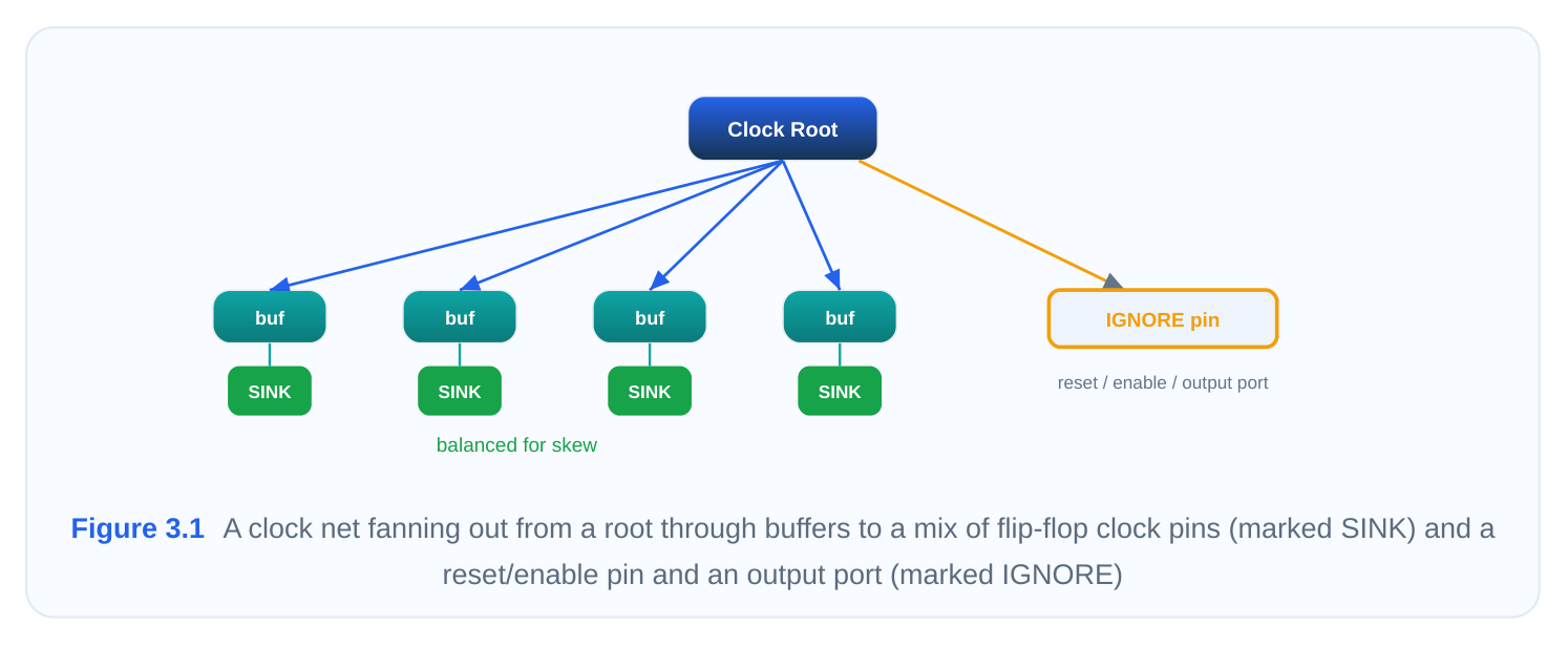
Before a CTS engine can build anything, it has to answer one deceptively simple question: where does the clock need to arrive, and where does it not matter? Every pin that the clock net touches falls into one of two buckets. Either it is a destination the tool must service and balance (a sink), or it is a point the tool should route to but never balance against (an ignore pin). Getting this classification right is the difference between a tree that closes timing and one that fights you for weeks.
3.1.1 Sink Pins / Balanced Endpoints
A sink pin is any clock endpoint the tool is responsible for delivering the clock to and balancing. These are the points that define skew. When the engine computes how to distribute buffers and equalize delay, it is measuring delay to the sinks and trying to make those delays as equal as possible. The classic sinks are:
- Flip-flop and latch clock inputs. The
CKorCLKpin of every sequential element driven by the clock. This is the bread and butter of CTS, because flop-to-flop paths are exactly where skew directly trades against setup and hold slack. - Macro clock pins. Hard macros, memories, and IP blocks expose a clock pin. Even though you cannot see inside the macro, that pin is a real load and a real timing endpoint, so the tool balances to it. Macros often carry large internal insertion delay, which makes them important pins to handle carefully (more on that under insertion delay).
- Active balancing points. Any user-declared point that should participate in skew equalization. Sometimes you deliberately promote a pin to sink status so the tool equalizes delay to it even though, by default, the tool would have ignored it. Two properties define how the tool treats a sink. First, it gets a zero insertion-delay assignment by default, meaning the tool assumes no additional delay budget sits beyond that pin and it tries to land the clock edge there at the same time as every other sink. Second, the sink is a skew-minimization endpoint: it is one of the leaves whose arrival times the engine is actively driving toward each other. If you have 50,000 flops, you effectively have 50,000 sinks (grouped into balancing sets), and the global skew number you report is computed across them. The mental model: sinks are the pins where the clock edge actually launches or captures data, so the tool must make them arrive together.
3.1.2 Ignore Pins / Excluded From Balancing
An ignore pin is a pin on the clock net that the tool will route to so the net is electrically complete, but which it deliberately leaves out of skew balancing. The clock still physically reaches the pin; the tool just does not try to equalize its delay against the sinks. Ignoring is not the same as not connecting. Common ignore pins:
- Output ports feeding cascaded clocks. When a clock leaves the block through an output port to drive another block's clock tree, the port itself should not be balanced as if it were a flop. The downstream block owns its own balancing. Treating it as a sink would force the tool to add or remove delay for a pin whose real budget it cannot see.
- Non-clock functional inputs. Reset, set, clear, scan-enable, and similar control pins sometimes get fed by a clock-derived or test signal. They are not timing-critical against the clock the way a flop CK pin is, so balancing to them is pointless and can distort the tree.
- Data inputs accidentally on the clock net. If a clock net (or a divided/gated version) reaches a
Dpin or a logic input, you do not want to balance to it. - Three-state enable pins. The enable of a tri-state buffer driven from clock logic is a control point, not a capture point.
- Source pins of other clocks. When one clock's net touches the generation point (the master source) of a different, downstream generated clock, that point belongs to the second clock's tree. The first tree should ignore it and let the generated clock's own CTS handle balancing.
- Isolation with guide buffers. A subtle but important use: by declaring a point an ignore pin and inserting a guide buffer (a buffer the tool is told to keep and build through), you isolate one portion of the network so it does not perturb the balancing of another. The guide buffer acts as a clean handoff boundary. The mental model: ignore pins are along for the ride electrically, but they are invisible to the skew cal‐ culation.
3.1.3 Endpoint Identification
How does the tool decide which pins are sinks and which are ignored? It runs an automatic deriva‐ tion based on the timing graph and library information. Starting from the clock root, the engine traces the clock net, looks at each pin it reaches, and uses the cell's .lib timing arcs to classify it. A pin with a setup/hold timing arc relative to the clock (a real sequential clock pin) becomes a sink. A pin that is purely a data or control input, or a port, defaults to ignore. This auto-classification is good but not infallible. Library modeling gaps, unusual cell types, custom macros, and creative clocking schemes all produce cases where the tool guesses wrong. That is why design-specific overrides exist: you can force a pin to be treated as a sink or as an ignore pin regardless of what the tool inferred. These overrides are the bridge to the next section, clock tree ex‐ ceptions.
Finally, verification is non-negotiable. Before letting CTS run for hours, dump the clock structure and confirm the sink and ignore lists match your intent. A few quick reporting commands save enormous grief.
# Inspect how the tool has classified clock endpoints
report_clock_tree -summary
report_clock_timing -type skew -clock CLK
# List the sinks the tool intends to balance for a given clock
get_clock_tree_pins -clock CLK -sink
# Sanity-check which pins are being ignored
report_ignored_pins -clock CLK
The single most common rookie mistake here is assuming the default classification is correct on a block with macros or custom clock gating. Always verify.
3.2 Clock Tree Exceptions
Exceptions are how you tell the tool, "I know better than your defaults for this specific pin." They are the controlled overrides on top of automatic endpoint identification. There are three flavors that matter for interviews: promoting a pin to a sink, demoting a pin to ignore, and imposing an insertion-delay re‐ quirement.
3.2.1 User-Defined Sink Pins
Sometimes the tool's auto-derivation leaves a pin as an ignore pin, but you genuinely want the clock balanced to it. The classic case is a custom or poorly modeled cell whose clock input does not carry a recognizable timing arc, so the tool never promoted it. You convert it from ignore to sink so it joins the balancing set.
# Promote an auto-ignored pin so the tool balances the clock to it
set_clock_balance_points \
-consider_for_balancing true \
-pins [get_pins custom_macro/CK_INT]
Once promoted, that pin is now part of the skew calculation. Its arrival time will be driven toward the rest of the sinks, the tool will spend buffers to make that happen, and your reported skew will include it. Use this when a real capture point is being silently excluded.
3.2.2 User-Defined Ignore Pins
The opposite move: the tool wants to balance a pin, but you know it should not be balanced. Maybe it is a port to another block, a clock-derived reset, or a point you want to isolate. You demote it to ignore.
# Demote a pin so the tool routes to it but excludes it from skew balancing
set_clock_balance_points \
-consider_for_balancing false \
-pins [get_ports CLK_OUT]
A related and powerful technique is forcing guide buffers at an ignore boundary. By declaring the handoff point an ignore pin and instructing the tool to build a specific buffer there, you create a clean, predictable interface. The guide buffer absorbs the upstream drive and presents a known load and known delay to whatever is downstream, so the two regions can be optimized independently without one corrupting the other's balancing. The discipline to remember: ignoring a pin removes it from skew math, but it does not remove the physical load. The tool still has to drive it. So an ignore pin with a huge load still needs adequate buffering for transition, even though it is not a balancing target.
3.2.3 Insertion Delay Requirements
The third exception type sets a required insertion delay at a point rather than just including or ex‐ cluding it from balancing. This is essential for phase delay management and for multi-parent gener‐ ated clocks. Consider a generated clock (say a divide-by-2) whose source has a known insertion delay from the master clock's tree. The generated clock's own tree needs to start its budget accounting from that point, not from zero. If you let the tool treat the generation point as a zero-delay sink, the two trees will not line up and you will see phantom skew between the parent and child clock domains. Multi-parent situations are worse: a generated clock can be reachable through more than one master source, each arriving with a different delay. To reconcile them, you tell the tool the target insertion delay so all parents converge to a consistent number at the handoff.
# Impose a target insertion delay at a generated-clock source point
set_clock_balance_points \
-delay 0.180 \
-pins [get_pins clk_div/Q]
# Combine: keep balancing AND pin a delay target
set_clock_balance_points \
-consider_for_balancing true \
-delay 0.180 \
-pins [get_pins clk_div/Q]
The table below summarizes the three exception types and when each applies.
Exception
Command intent When you use it Effect on balancing
| User-defined | -consider_for_balancing | A real capture/clock pin the | Added to skew set; |
|---|---|---|---|
| sink | true | tool wrongly ignored | delay equalized |
| User-defined | -consider_for_balancing | Ports, control pins, isolation | Routed but excluded |
| ignore | false | points | from skew |
| Insertion- | -delay <value> delay target | Phase delay, multi-parent generated clocks | Forces a specific arrival, aligns domains |
3.3 Design Rule Constraints
Design Rule Constraints, or DRCs, are the electrical guardrails CTS must respect while it builds. They are not optional optimization goals; they are hard limits on capacitance and transition that keep the clock signal clean and the tree physically buildable. They also have an outsized, sometimes counterin‐ tuitive effect on how many buffers the tool inserts and how the tree is shaped.
3.3.1 Maximum Capacitance
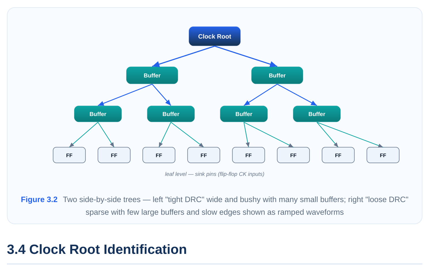
max_capacitance caps the total load that any single clock buffer's output may drive. A typical default sits around 0.55 pF, though the real number is technology- and cell-dependent. The purpose is twofold: protect against degraded slew (a buffer overloaded with capacitance produces a slow, sloppy edge) and bound the load per driver so signal integrity stays in spec. When a region of the tree carries more load than one buffer can legally drive, the constraint forces the tool to distribute the load across multiple buffers. This is the direct mechanism that grows the tree's width: a tight cap means each buffer drives fewer sinks, which means more buffers in parallel, which means more levels and more area, but cleaner edges.
# Constrain per-driver load on the clock network
set_max_capacitance 0.480 [get_clocks CLK]
# Apply to the whole current design as a ceiling
set_max_capacitance 0.550 [current_design]
The trade-off is real: lower the cap and you spend buffers and power for better edges; raise it and you save area but risk slew violations and weaker drive.
3.3.2 Maximum Transition Time
max_transition caps the slew (rise/fall time) of the clock signal at any pin. A common default is around 0.45 ns, and again the practical value depends on the process node and how aggressive the clock is. Where max_capacitance constrains the cause (load), max_transition constrains the
symptom (edge speed). They are related but not identical, and a tight transition limit is often the dominant driver of buffer count on high-speed clocks. Why transition matters so much for clocks: a slow clock edge stretches the window during which the receiving flop is uncertain, increases delay variability, and is a notorious contributor to hold violations because slow edges interact badly with short data paths. Keeping clock slew crisp is one of the most direct levers on robust timing. The constraint can be specified separately for rising and falling edges when a technology has asym‐ metric drive. Meeting a tight transition target frequently pushes the tool to pick stronger (higher drive- strength) buffers rather than just more of them, because a beefier buffer produces a faster edge into the same load.
# Cap clock slew on the network
set_max_transition 0.320 [get_clocks CLK]
# Separate rise/fall limits where the library supports it
set_max_transition 0.280 -rise [get_clocks CLK]
set_max_transition 0.280 -fall [get_clocks CLK]
3.3.3 Constraint Trade-offs
There is no universally "correct" DRC setting. It is a deliberate trade between timing quality, power, and area, and a good engineer tunes it to the clock's importance.
| Setting | Buffer count & | ||||
|---|---|---|---|---|---|
| max_cap / max_tran | Power | Timing quality | Risk | ||
| style | area | ||||
| Tight | Low (e.g. 0.25 pF / | High | Higher | Best edges, low | Area/power |
| 0.22 ns) | skew | blowup | |||
| Moderate | Default (~0.55 pF / | Balanced | Bal‐ | Good | Reasonable de‐ |
| 0.45 ns) | anced | fault | |||
| Loose | High (e.g. 0.85 pF / | Low | Lower | Weaker edges | Slew & hold viol‐ |
| 0.75 ns) | ations |
The instinct an interviewer wants to see: tight constraints buy you better timing and signal integ‐ rity at the cost of more buffers, more area, and more clock power, while loose constraints save resources but risk slow edges, larger skew, and hold problems. On the highest-frequency clock in a chip you bias tight; on a slow, sleepy peripheral clock you can afford to relax and save power. Typical production ranges keep transition somewhere in the few-hundred-picosecond region for fast clocks and let capacitance ride near the technology default unless slew analysis says otherwise.
Every clock tree has to start somewhere, and the clock root is that starting point: the node from which the tool fans out and against which it measures insertion delay. Identifying roots correctly is founda‐ tional, because a misidentified root means the tool balances the wrong network or misses an entire domain. Roots come in several forms:
- Primary input clock ports. The most common root is a top-level clock pin where the clock physic‐ ally enters the chip from a PLL output or an external oscillator. This is where
create_clockis ap‐ plied and where insertion delay is measured from. - Internal hierarchical pins. In a block-level or hierarchical flow, the clock may enter not at a chip pad but at a block boundary pin. That boundary pin is the root for that block's tree even though it is internal to the full chip.
- Generated-clock master sources. A generated clock (divided, multiplied, gated, or muxed) is defined relative to a master pin. That master/source pin is the root of the generated clock's own subtree. The tool must recognize it so the generated clock gets its own balanced tree starting from the right place.
- Nested clock tree roots. Clocks can stack: a generated clock can itself be the master of a further generated clock. Each level introduces a new root nested inside the previous tree. Recognizing the hierarchy of roots is what lets the tool build each subtree with the correct delay budget and avoid double-counting or skipping delay.
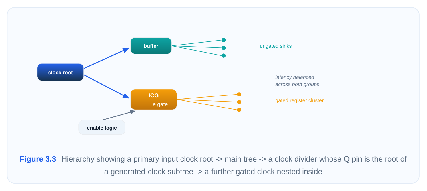
The practical workflow is to enumerate every clock object, confirm the tool resolved each root to the pin you expect, and check that generated clocks point back to the right master.
# Enumerate all clocks and their source/root objects
report_clocks
foreach_in_collection clk [all_clocks] {
puts "[get_object_name $clk] -> [get_attribute $clk sources]"
}
# Confirm a generated clock's master source (its root)
report_clock -generated [get_clocks CLK_DIV2]
If a root resolves to an unexpected pin, stop and fix the constraints. Building a tree from the wrong root wastes the entire run.
3.5 Clock Tree Structure
With endpoints, exceptions, constraints, and roots understood, you can finally picture the object CTS produces: a buffered distribution network from root to sinks. Its structure has a vocabulary every PD engineer should own.
Tree Depth and Levels
Depth is the number of buffer stages between the root and the farthest sink. A clock that passes through, say, root → buffer → buffer → buffer → flop has a depth of three buffer levels. Depth is a balancing act: a deeper tree spreads load gracefully and keeps each stage's slew clean, but every extra level adds insertion delay and, critically, adds variation because each buffer contributes its own process/voltage/temperature spread (OCV). Shallower trees have less insertion delay and less accu‐ mulated variation but stress each stage harder. Modern flows fight to keep depth low precisely to cut OCV-driven skew.
Buffer Hierarchy
The tree is organized as a hierarchy of buffers: a small number of large drivers near the root handle the bulk fan-out, and progressively the load is split among more, often smaller, buffers as you approach the leaves. This staged splitting is exactly what the max_capacitance and max_transition constraints enforce — each level exists to keep its drivers within DRC while passing a clean edge to the next level.
| Tree region | Typical role | Buffer characteristics |
|---|---|---|
| Root / top levels | Bulk fan-out from the source | Few, large, high-drive buffers |
| Mid levels | Load distribution | More buffers, moderate drive |
| Leaf level | Final delivery to sinks | Many small buffers, short nets |
Leaf-Level Sinks
The leaf level is where the clock finally reaches the sink pins identified back in section 3.1 — the flop CK pins and macro clock inputs. The last buffer before a cluster of sinks is the leaf driver, and the quality of the edge it delivers (its transition) directly sets capture-side timing. Leaf clusters are usually formed by grouping physically nearby sinks so each leaf driver sees short routes and low load.
Convergence Patterns
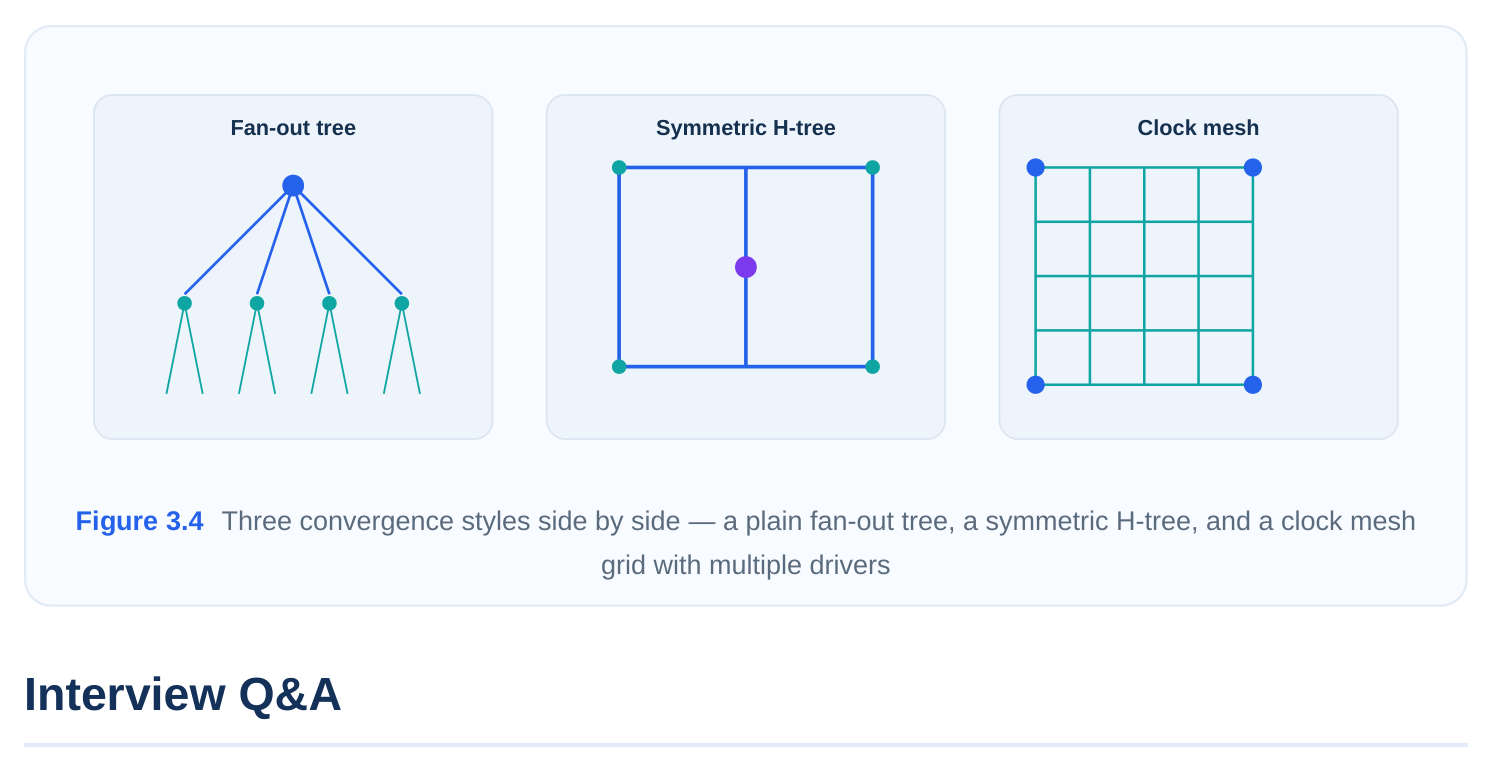
A simple tree diverges from root to leaves and never rejoins — a pure fan-out. But real clock distribution often uses convergence structures to crush skew. The two patterns worth naming:
- H-tree / balanced tree. A geometrically symmetric structure where every path from root to leaf traverses the same nominal length and the same number of buffers. Symmetry makes nominal skew near zero by construction. H-trees are common for top-level, high-performance clock spines.
- Clock mesh / grid. Instead of (or above) a tree, a metal grid shorts together many drivers so the clock arrives nearly simultaneously everywhere on the mesh. Meshes deliver outstanding low skew and excellent variation tolerance at the cost of significant power and routing resources, so they appear mostly on the most aggressive, highest-frequency designs. Most real chips blend approaches: a balanced spine or mesh at the top for the critical domain, conven‐ tional buffered trees for the rest. Recognizing which convergence pattern a design uses tells you a lot about how aggressively it is chasing skew.
pin disconnect it? A sink pin is a clock endpoint the tool both routes to and balances — its delay is part of the skew calculation, and the engine spends buffers to equalize it with other sinks. An ignore pin is still physically driven and routed (the clock reaches it), but it is excluded from skew balancing. Ignoring does not disconnect the pin and does not remove its electrical load; the tool still must satisfy transition and capacitance to it. The distinction is purely about whether the pin participates in skew math.
it, and what changes as a result? The tool auto-classified that pin as an ignore pin, likely because the library cell lacks a recognizable clock timing arc. Promote it with
set_clock_balance_points -consider_for_balancing true on that pin. Afterward, the pin joins thebalancing set: its arrival time is driven toward the other sinks, the tool may add buffering to align it, and your reported skew now accounts for it. The risk is that a far-off or heavily loaded promoted sink can pull the whole tree and increase insertion delay, so verify the result.
clock edges widen timing uncertainty at the capture flop and interact badly with short data paths, which is a classic source of hold violations. Tightening max_transition forces crisper edges — usually by inserting more buffers or selecting stronger drivers — which reduces that uncertainty and the variability that feeds hold problems. The cost is more buffers, more clock power, and more area; on a non-critical clock that overhead may not be worth it, so the setting is tuned per clock.
with different delays. How do you make the domains line up? This is a multi-parent generatedclock situation. Use an insertion-delay requirement at the generation point with set_c‐ lock_balance_points -delay <value> so the tool drives both parent paths to converge on the same arrival at the source pin. Without this, the two parents land at different times and you see phantom
skew between the parent and child domains. Pinning the target insertion delay reconciles the phase relationship across the handoff.
like H-trees or meshes help? Each buffer stage adds insertion delay and, more importantly, adds its own PVT/OCV variation, so a deep tree accumulates variation that shows up as skew under on-chipvariation analysis. Keeping depth low reduces that accumulated spread. Convergence structures attack skew differently: an H-tree makes every root-to-leaf path geometrically and electrically symmetric so nominal skew is near zero by construction, while a clock mesh shorts many drivers together so the edge arrives almost simultaneously everywhere. Both buy very low skew and strong variation tolerance, at the price of power and routing resources, which is why they appear on the most aggressive clocks.
Key Takeaways
- Sinks are balanced, ignore pins are not — but ignore pins are still routed and still impose elec‐ trical load, so DRCs apply to them regardless.
- Endpoint classification is auto-derived from library arcs and is fallible; always verify the sink and ignore lists before a long CTS run, especially on designs with macros or custom clocking.
- Exceptions are your override layer:
-consider_for_balancing true/falsepromotes or de‐ motes pins, and-delaypins a required insertion delay for phase alignment and multi-parent generated clocks. - max_capacitance bounds load per driver and max_transition bounds slew; together they are the primary force that determines how wide and how deep the tool builds the tree.
- DRC tuning is a deliberate trade-off — tight settings buy timing and signal-integrity quality at the cost of buffers, power, and area; loose settings do the reverse and risk slew and hold violations.
- Roots come in several forms (primary clock ports, hierarchical boundary pins, generated-clock masters, and nested roots), and a misidentified root wastes the entire build.
- Low depth reduces accumulated OCV-driven skew, and convergence structures like H-trees and meshes drive nominal skew toward zero by symmetry or by shorting drivers together, at a power and routing cost reserved for the most critical clocks.
Comments
Leave a Reply