 ChipBuddy
← Home
ChipBuddy
← Home
Clock-Tree Design-Rule Constraints
Clock tree synthesis lives and dies by its design rule constraints. You can have the cleanest skew target in the world, but if the buffers you drop into the tree are driving loads they were never characterized for, the resulting clock waveform degrades into something the timer can no longer trust. Two constraints sit at the center of this discipline: maximum capacitance and maximum transition. Together they define the electrical envelope inside which every clock buffer, inverter, and net must operate. This topic walks through both constraints in depth, how they interact, how to apply them percorner and per-mode, and how the tool reacts when it has to honor them.
7.1 Maximum Capacitance Constraint
7.1.1 Definition and Impact
The maximum capacitance constraint puts a ceiling on the total load that any driving pin in the clock network is allowed to see. That load is the sum of the wire capacitance of the net plus the input pin capacitances of every cell the net fans out to. When a buffer or inverter drives more capacitance than the rule permits, you have a max_cap violation. Why does this matter so much in a clock tree? A clock buffer is a transistor-level circuit that was characterized in the standard cell library across a specific range of output loads. The library timing arcs, the delay tables, the output slew tables, all of them are valid only within that characterized load
window. Push the buffer past its intended load and you are extrapolating off the edge of the model. Two bad things happen physically. First, the output edge rate collapses, the rise and fall times stretch out because the same drive current is now charging and discharging a larger capacitor. Second, the cell delay balloons and becomes increasingly nonlinear, which makes skew balancing unreliable.
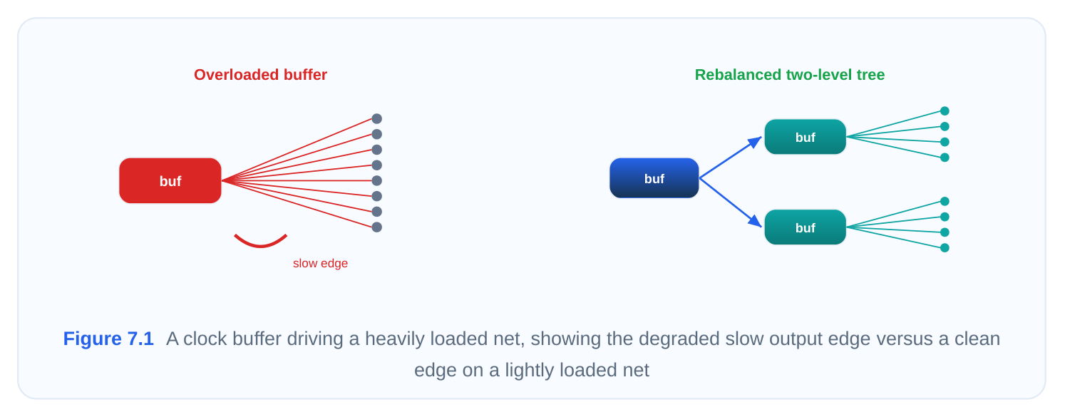
So the maximum capacitance rule is really a proxy for protecting drive capability and, indirectly, for keeping slew under control. It says: never let a driver work harder than the silicon was designed to. In practice, max_cap is the constraint that most directly governs how many sinks a single buffer can fan out to before CTS must split the load. It is your first line of defense against slew violations, because slew degradation is downstream of overload, and it is the constraint that shapes the branching factor of the entire tree.
7.1.2 Implementation
The command used across most implementation flows is set_max_capacitance . It attaches a capa‐ citance ceiling to a design object, a port, a pin, a clock, or the whole design, and the engine treats any net whose driver exceeds that value as a violation to be fixed. You can apply it globally, which sets a blanket rule for everything, or scope it tightly to the clock network so that the clock obeys a stricter limit than the datapath. Scoping to a clock is the common practice because clock nets demand cleaner edges than ordinary signal nets.
# Global ceiling applied to the entire current design
set_max_capacitance 0.55 [current_design]
# Stricter ceiling applied only to objects of a named clock
set_max_capacitance 0.35 [get_clocks core_clk]
# Apply to specific clock root pins / ports
set_max_capacitance 0.42 [get_ports CLK_IN]
Units matter. In most timing engines the capacitance unit is inherited from the technology library, and for modern nodes that unit is picofarads (pF). Always confirm with report_units before you trust a number you typed. A value of 0.6 may be 0.55 pF or, in a library configured for femtofarads, a wildly
different magnitude. Getting the unit wrong is one of the most common silent constraint mistakes engineers make.
# Confirm the library capacitance unit before setting values
report_units
When you load constraints, the tool stores max_cap as an attribute on the affected objects, and you can query the effective value with attribute reporting to make sure a global setting was not unintentionally overridden by a tighter per-clock value.
7.1.3 Constraint Values
There is no single universal number, because the right ceiling depends on the standard cell library, the process node, the metal stack, and how aggressive the timing closure needs to be. That said, real flows cluster around recognizable ranges. The table below gives representative starting points.
| Setting | Typical max_cap value | When to use it |
|---|---|---|
| Tight | 0.35 pF | Aggressive slew targets, high-frequency clocks, advanced nodes |
| Default | 0.55 pF | Balanced starting point for most CTS runs |
| Loose | 0.95 pF | Lower-frequency clocks, area/power-sensitive blocks, relaxed slew |
A tighter ceiling forces the tool to keep buffers lightly loaded, which produces sharper edges and lower skew but at the cost of more buffers, more area, and more dynamic power. A looser ceiling lets each buffer absorb more sinks, shrinking the tree but risking slower edges. The default sits in the middle and is where most teams begin before tuning. The next table shows how these targets typically shift with technology node, since smaller geometries pull the ceiling down.
| Process node | Common clock max_cap range |
|---|---|
| 28 nm and above | 0.45 to 0.95 pF |
| 16 / 14 nm | 0.25 to 0.55 pF |
| 7 nm and below | 0.08 to 0.25 pF |
These are illustrative. Always defer to the values your library vendor and CTS reference methodology recommend, then refine based on post-CTS slew and skew reports.
7.1.4 Tool Behavior
When CTS encounters a node whose load exceeds the max_cap ceiling, it does not simply flag it and move on, it actively restructures the tree to fix it. The dominant mechanism is buffer insertion. Instead
of one driver fighting an oversized load, the engine inserts additional buffers so the load is split across multiple drivers, each one sitting comfortably inside its characterized window.
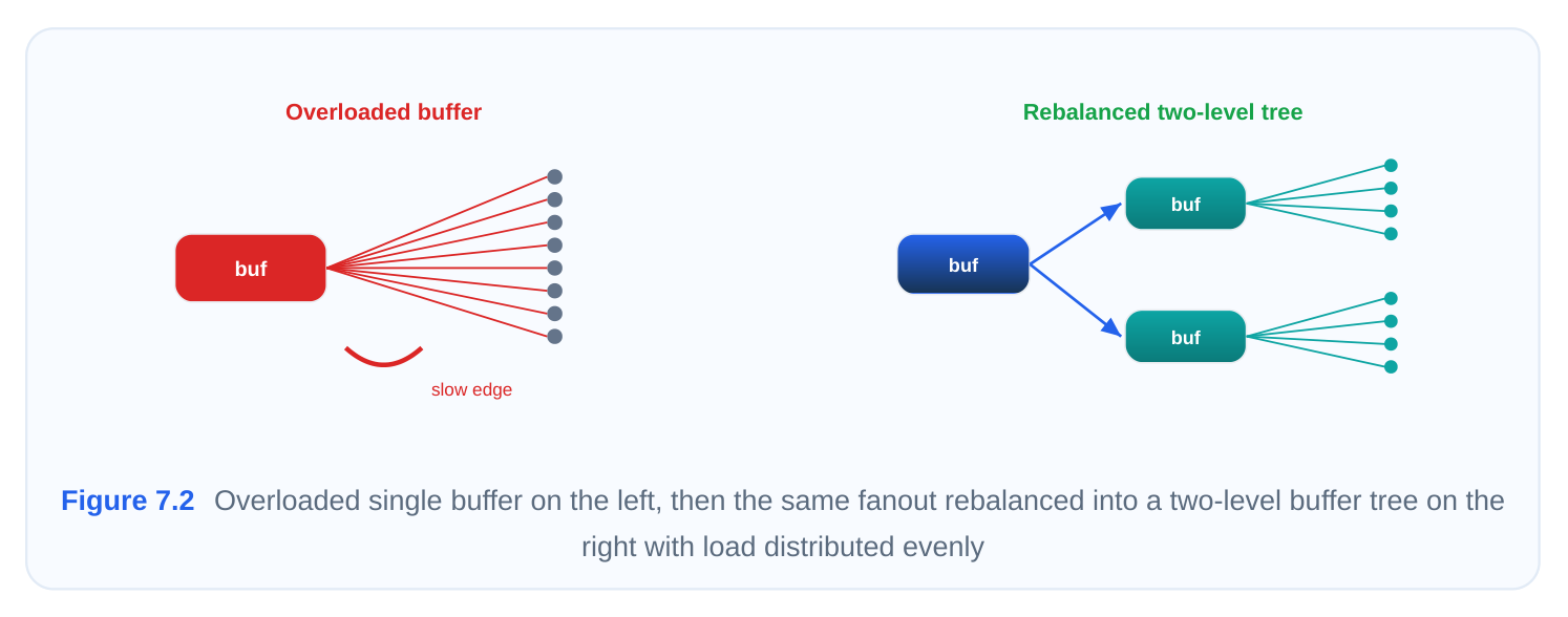
Several behaviors follow from this:
- Multi-buffer insertion. A heavily fanned-out node gets subdivided. The tool may insert a layer of intermediate buffers, each driving a fraction of the original sinks, until every driver is under the ceil‐ ing.
- Load distribution. The engine tries to balance the number of sinks per branch so that no single buffer is near the limit while its sibling sits half-empty. Even distribution helps skew as well as max_cap.
- Buffer-tree restructuring. Fixing one violated node can change the load on its parent, so CTS iterates, rebuilding levels of the tree until the whole network is clean. This is why max_cap directly drives tree depth and branching factor.
- QoR impact. Every buffer added to satisfy max_cap costs area and power, and each extra level of buffering adds insertion delay and another source of on-chip variation. A ceiling set too tight inflates buffer count and power; set too loose, you trade those savings for slew and skew risk. The art is finding the value that closes timing with the fewest cells.
7.2.1 Definition and Impact
Transition time, also called slew, is how long a signal takes to swing between defined voltage thresholds, typically from 10 percent to 90 percent of the supply on a rising edge and the reverse on a
falling edge. The maximum transition constraint caps how slow that swing is allowed to be on any clock pin or net. Exceed it and you have a max_transition violation. Where max_cap protects the driver, max_transition protects the waveform itself, and it is enforced at the receiving end. A slow clock edge is corrosive in several ways. It increases the cell's effective propagation delay and makes that delay sensitive to noise and process variation, because the receiv‐ ing flop's clock pin spends longer in its uncertain switching region. It widens the window during which crosstalk can nudge the edge earlier or later, degrading timing predictability. And critically, sluggish clock slews are a frequent root cause of hold violations, because the relationship between launch and capture edges depends on consistent, sharp transitions across the tree.
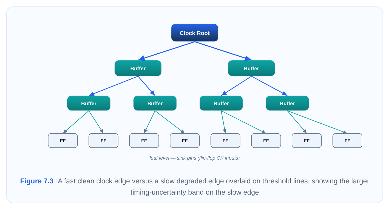
This is why clock nets are held to far stricter transition limits than data nets. A clean, fast, uniform slew everywhere in the clock network is the foundation of trustworthy skew numbers and robust setup and hold margins.
7.2.2 Implementation
The constraint is applied with set_max_transition . Like its capacitance counterpart, it can be global or scoped, and scoping it to the clock object is the standard way to give the clock a tighter rule than the rest of the design.
# Tight transition ceiling for a specific clock
set_max_transition 0.135 [get_clocks core_clk]
# Global transition rule for the whole design
set_max_transition 0.45 [current_design]
# A clock-network-specific form available in many flows
set_max_transition 0.11 -clock_path [get_clocks core_clk]
Units here are time, almost always nanoseconds (ns) in modern libraries, though again you should verify with report_units . Many CTS flows also support a dedicated clock-transition option so that the clock path can carry a different slew target from data paths sharing the same pins, which is essential when a pin is reached by both clock and signal propagation. A subtle point worth knowing for interviews: when both a library-defined slew limit (from the cell's max_transition attribute in the .lib) and a user set_max_transition exist, the tool generally honors the more restrictive of the two. Your SDC value cannot loosen a hard library limit, it can only tighten the effective constraint.
7.2.3 Constraint Values
Transition targets are even more technology-bound than capacitance targets, because slew scales with device speed and supply voltage. The table below shows representative clock slew ceilings.
| Setting | Typical max_transition value | Character |
|---|---|---|
| Tight | 0.13 ns | High-speed clocks, advanced nodes, strict skew budgets |
| Default | 0.27 ns | Common balanced clock target |
| Loose | 0.45 ns | Relaxed, lower-frequency or power-sensitive clocks |
A useful rule of thumb that interviewers like to hear: clock transition is often budgeted as a small fraction of the clock period, frequently in the range of 5 to 10 percent. So a 1 GHz clock with a 1 ns period would target a slew well under 0.09 ns, while a slower clock can tolerate a relaxed limit. The next table illustrates that period relationship.
| Clock frequency | Period | Reasonable clock slew target |
|---|---|---|
| 200 MHz | 4.8 ns | up to ~0.27 ns |
| 500 MHz | 2.4 ns | ~0.15 to 0.18 ns |
| 1 GHz | 0.95 ns | ~0.08 to 0.11 ns |
Keep the clock transition limit meaningfully tighter than the data transition limit. A frequent default split is something like 0.13 ns for clock pins against 0.4 to 0.45 ns for data, so that the clock always presents the cleanest edges in the design.
7.2.4 Tool Behavior
When CTS sees a clock pin whose transition exceeds the limit, its primary lever is buffer-strength optimization. Rather than always adding more buffers as it does for max_cap, the tool can swap in a stronger drive-strength variant of the same cell, a buffer with wider transistors that pushes more current and therefore sharpens the edge driving the same load.
Key behaviors:
- Buffer-strength optimization (sizing). Upsizing the driver is the first response to a slow edge. A 2x buffer replaced by a 4x or 7x version drives the existing load faster, pulling the transition back inside the ceiling.
- Combined with insertion. When upsizing alone cannot meet the slew target, or when it would create a new max_cap problem on the upsized cell's own input, the tool falls back to inserting buffers and splitting the load, the same restructuring used for capacitance. The two fixes are deeply intertwined.
- Slew-violation resolution order. Tools generally resolve max_cap first, then check transition, because fixing the load often fixes the slew for free. Residual transition violations are then mopped up with targeted sizing.
- Timing-margin maintenance. Throughout this, the engine is trying not to wreck skew or insertion delay. Aggressive upsizing adds input load upstream and can shift delays, so the optimizer balances slew repair against the skew and latency targets it must simultaneously honor.
Max_cap and max_transition are not independent dials, they are two views of the same physical phe‐ nomenon, and tuning one moves the other. Understanding their interplay is what separates someone who copies default constraints from someone who can actually close a clock tree.
The capacitance versus transition trade-off
A driver's output slew is fundamentally a function of its drive strength and the load it carries. If you tighten max_cap, you force smaller loads per driver, which naturally improves slew, often to the point where max_transition violations disappear on their own. Conversely, if you tighten max_transition without touching max_cap, the tool responds by upsizing drivers, which increases the upstream input capacitance those drivers present to their parents, potentially creating new max_cap violations one level up. The two constraints chase each other through the tree.
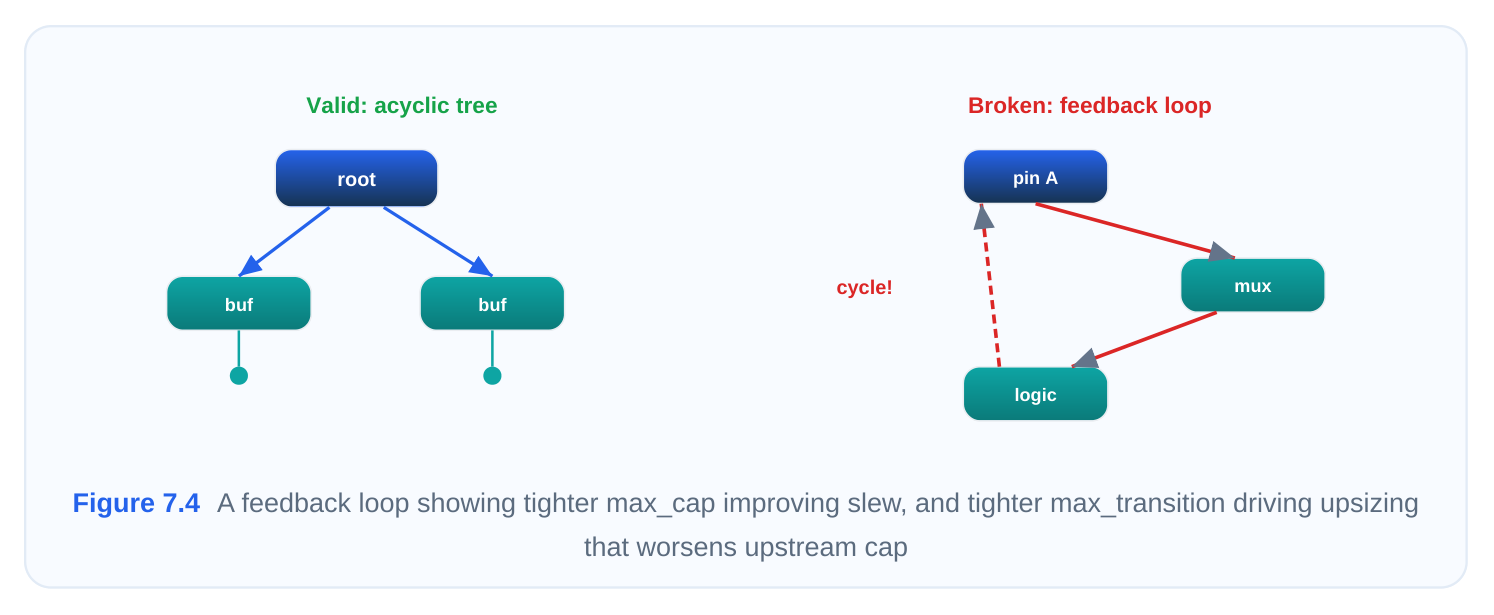
This coupling means the constraints must be set as a consistent pair. A max_transition target that no buffer in the library can achieve at the allowed max_cap is simply infeasible, and the tool will either churn endlessly or leave violations. A good sanity check: pick a target slew, find the library buffer that hits it, and confirm the load it can drive at that slew is at or above your max_cap ceiling.
Buffer sizing and tree depth
The two main repair levers, inserting more buffers versus upsizing existing ones, push tree topology in opposite directions. Insertion adds breadth and depth, more cells across more levels. Upsizing keeps the level count flat but grows individual cell sizes. Tight max_cap pushes toward deeper, bushier trees with more levels because each driver handles fewer sinks. Tight max_transition with loose max_cap pushes toward fewer, larger buffers. Most real trees land somewhere in between, and CTS continu‐ ously chooses between the two based on which fix is cheaper at each node.
Power, timing, and area trade-offs
Every choice ripples into the classic three-way trade-off.
| Constraint change | Effect on power | Effect on timing/skew | Effect on area |
|---|---|---|---|
| Tighten max_cap | Higher (more buffers | Better slew, often better skew switch) | Larger (more cells) |
| Loosen max_cap | Lower | Risk of slew degradation | Smaller |
| Tighten max_trans‐ | Higher (bigger/more buf‐ ition | Sharper edges, better hold robust‐ fers) | Larger ness |
| Loosen max_trans‐ | Lower | More timing uncertainty | Smaller |
ition The clock tree is typically one of the largest dynamic power consumers on a chip, often a double-digit percentage of total switching power, so over-tightening these rules has a real power cost. The
discipline is to set the loosest constraints that still deliver the slew and skew your timing signoff requires, no tighter. Closing timing with the minimum buffer count is the mark of a well-tuned tree.
7.4 Constraint Propagation
Setting a constraint once is not enough. A real design is analyzed across many process-voltage-tem‐ perature corners and many functional modes, and the constraints have to be present and correct in every one of them, or signoff will miss violations that only appear under specific conditions.
Across all corners
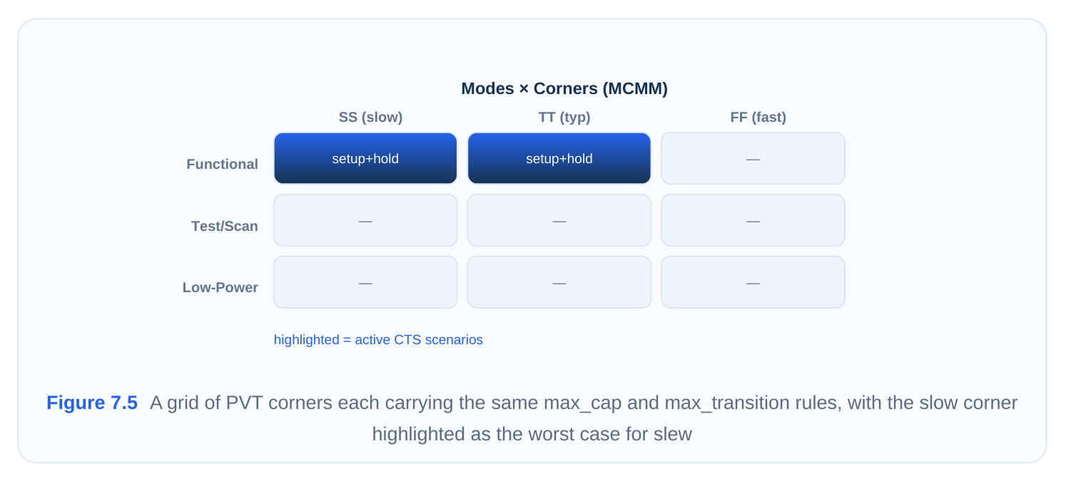
A clock buffer behaves very differently in a slow corner (slow process, low voltage, high temperature) than in a fast corner. Slew degrades worst in the slow corner, while max_cap headroom can be tight‐ est there too. If your constraints are only loaded in the typical corner, the tool optimizes for typical and the slow-corner slews blow past their limits in signoff. Best practice is to ensure
set_max_capacitance and set_max_transition are active in the constraint set used for every ana‐lysis corner, and to validate violations corner by corner.
Across all scenarios and modes
Modern flows use multi-mode multi-corner (MMMC) analysis, where a scenario pairs a mode (function‐ al, test, scan, low-power) with a corner. Each mode can legitimately need different clock constraints. A scan or test mode may run the clock slower and tolerate a looser slew, while functional mode demands the tight limit. Mode-specific constraints let you express that.
# Functional mode: strict clock rules
set_max_transition 0.11 [get_clocks core_clk] ;# in func scenario constraints
set_max_capacitance 0.35  [get_clocks core_clk]
# Test/scan mode: relaxed because the shift clock runs slower
set_max_transition 0.36 [get_clocks scan_clk]
set_max_capacitance 0.75  [get_clocks scan_clk]
In an MMMC setup these are bound to the appropriate analysis views so that each scenario applies its own rules. The CTS engine then optimizes the tree to satisfy the union of all active scenarios, which means the tightest applicable constraint at any node wins.
Override mechanisms
Constraints stack, and when multiple apply to the same object the most specific and most restrictive one governs. A few practical mechanisms:
- Scope precedence. A constraint set on a specific pin or clock overrides a broader one set on the whole design for those objects, but only in the direction of being more specific, not necessarily more permissive.
- Tighter-wins for slew. Where a library
max_transitionand a user value both exist, the engine honors the stricter one. Your SDC tightens, it does not loosen, a hard library limit. - Removing a constraint. When you genuinely need to lift a constraint on an object, use the explicit removal command rather than setting a huge number, which keeps the constraint database clean.
# Make a constraint more specific for one critical clock rootset_max_transition 0.09 [get_pins clk_root/Z]# Cleanly remove an inherited ceiling from a special netremove_max_capacitance [get_nets analog_bridge_clk]The takeaway on propagation: constraints are only as good as their coverage. A perfectly chosen max_transition value that is missing from the slow corner or the functional scenario is worse than useless, because it gives a false sense of a clean tree while the real worst case goes unchecked. Verify, corner by corner and mode by mode, that every clock object carries the rules you intend.
Interview Q&A
trees need both? Max_capacitance limits the total load a driver pin may see and protects the driver from operating outside its characterized window, it is enforced at the driving end. Max_transition limits how slow a signal edge may be and protects waveform quality, it is enforced at the receiving pin. They are related, overload causes slow slew, but they are not identical: a driver can be within its cap limit yet still
produce a marginal slew under a weak corner, and a strong driver can meet slew while a tight cap rule still flags it for restructuring. Clocks need both because the cap rule shapes how the tree branches while the transition rule guarantees the edge quality that skew and hold margins depend on.
The tool's first move is to upsize drivers to sharpen the edge. Bigger buffers present more input capacitance to their parent nets, so you can push the violation upstream and trigger new max_cap problems one level up. You also burn more dynamic power and area, and excessive upsizing can per‐ turb insertion delay and skew. If the target is below what any library cell can achieve at the permitted load, the constraint becomes infeasible and the optimizer churns without closing. The fix is to set cap and transition as a coordinated pair grounded in actual library cell capability.
I would use mode-specific constraints in an MMMC setup, binding tight values, for example 0.35 pF cap and 0.11 ns slew, to the functional scenario, and looser values to the scan or test scenario because the shift clock typically runs much slower and does not need the same edge sharpness. Each scenario carries its own SDC, the CTS engine optimizes to satisfy the union of active scenarios, and the tightest applicable rule wins at any node. This avoids over-buffering the test clock just to meet a limit that only matters at functional speed.
and how do you address it? This is the classic corner-dependent slew failure. In the slow PVT corner the buffer drives less current, so the same load that was fine in the typical corner now produces an edge that exceeds the transition limit even though the capacitance value itself is unchanged and still legal. The cap rule cannot catch it because cap is a static load count, not an edge-rate measurement. To fix it, ensure the constraint set is loaded and analyzed in the slow corner, then let CTS resolve it by upsizing the driver or splitting the load, and confirm with a slow-corner transition report. The deeper lesson is that slew must always be validated in the worst (slow) corner, never just in typical.
Key Takeaways
- Max_capacitance caps the load on the driving end to protect drive capability; max_transition caps edge slowness at the receiving end to protect waveform quality. Clock nets get far stricter limits than data nets.
- Typical clock starting points are around 0.35 to 0.55 pF for max_cap and 0.15 to 0.27 ns for max_transition, tightening sharply at advanced nodes; always verify units with
report_unitsand confirm against your library. - The two constraints are coupled: tightening cap usually improves slew for free, while tightening transition drives upsizing that can create new cap violations upstream, so set them as a consistent pair.
- CTS resolves violations by inserting buffers (load splitting, the main lever for max_cap) and by upsizing drivers (the main lever for max_transition), trading off power, area, and tree depth against timing.
- Constraints must propagate across every corner and every mode; the worst slew almost always appears in the slow corner, and mode-specific values let test clocks stay relaxed while functional clocks stay tight.
- The right answer is the loosest set of constraints that still meets signoff slew and skew, closing timing with the minimum buffer count to control clock power.
Comments
Leave a Reply