 ChipBuddy
← Home
ChipBuddy
← Home
What STA Is & Why It Replaced Simulation
Chapter 1 — What Static Timing Analysis Is, and Why It Replaced
Timing Simulation
Every clocked digital chip lives or dies by one question. Does each signal reach its destination flip-flop in time? It must arrive early enough to be captured safely. But it must not arrive so early that it wipes out the value the flip-flop still needs from the last cycle. A flip-flop (a tiny one-bit memory that updates on a clock edge) is the destination we care about. A modern design can have hundreds of millions of these checks. They must hold across every operating condition. Doing all that checking is the job of Static Timing Analysis (STA, a way to check chip timing without running the circuit). This chapter explains what STA actually computes. It also explains why the industry dropped pattern-based timing simulation for sign-off. And it introduces the timing graph, the mental model the rest of this handbook builds on.
The Core Idea: Timing Without Stimulus
The key word in "Static Timing Analysis" is static. STA never applies input patterns. It never toggles a single wire. It never runs the clock. Instead it treats the circuit as a map of delays. Then it asks a simple structural question. Given the worst delay along every possible path, can the data still make the trip in time?
STA does this by propagating arrival times forward through the design. An arrival time is the moment a signal reaches a pin. The tool starts the inputs and clock sources with known launch times. Then it walks the network of cells and wires. It adds each delay as it goes. Soon it knows the latest and earliest time a change can reach every pin. At each capturing flip-flop, it also computes a required time (the latest a signal is allowed to arrive and still be caught safely). The gap between required and arrival is the slack (how much timing margin is left):
slack = required_time − arrival_time (for a setup/max check)Positive slack means timing is met with room to spare. Negative slack means a violation. That one subtraction, run at every endpoint, is the heartbeat of STA. It helps to see why this works. Think of a clocked design as logic gates stitched together by registers. All the registers march to the same clock, like rowers following one drumbeat. Within one clock cycle, data leaves one register and must settle at the next register before it samples. STA puts numbers on this. It picks a launch edge that releases the data. It picks a capture edge that samples it. It computes how long the data really takes (the arrival). Then it compares that to how long the data is allowed to take (the required time). Setup checks ask "is the data fast enough?" They use the latest arrival. Hold checks ask "is the data not too fast?" They use the earliest arrival against the same capture edge. Every STA check is one of these two questions at one endpoint.
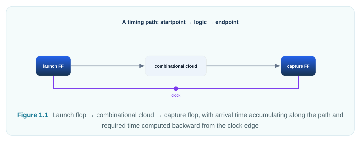
The big win is completeness. STA reasons about delays by structure, not by behavior. So it can guarantee it has checked every path between registers. It does not just check the paths some test happened to hit. A modern block can hold billions of distinct paths. STA covers all of them in one run, with no input patterns at all.
Static vs. Dynamic Timing Analysis
The old approach was dynamic timing analysis. You ran a gate-level logic simulation with real delays added (from an SDF file, which lists per-cell delays). Then you watched for timing violations as patterns flowed through. It worked. But it had two fatal flaws for large designs.
First, coverage is only as good as your patterns. A simulation only exercises the paths your input patterns happen to trigger. Suppose no pattern ever toggles the slowest path in your design. The simulator will happily report "no violations." Meanwhile a real silicon failure sits hidden, waiting. Getting even rough path coverage needs a huge, hand-built set of tests. And you can never be sure it is complete. Second, it is painfully slow. Gate-level simulation with delays can run far slower than real time. Now repeat that across many process, voltage, and temperature corners. A corner is one set of operating conditions. Sign-off then turns into a multi-week grind. It gets worse as gate counts grow. STA flips both problems. It needs no patterns, so coverage is built in and guaranteed. It does not depend on a clever test writer. And because it is a graph walk, not an event simulation, it is far faster. A full-chip run that simulation could never finish completes in reasonable time. Dynamic (Pattern-Based) Timing
Dimension Static Timing Analysis (STA)
| Stimulus needed | None — no patterns | Test patterns / testbench required |
|---|---|---|
| Path coverage | Complete (all structural paths) | Only paths the patterns trigger |
| Speed | Fast graph walk; scales to full chip | Very slow; event-driven simulation |
| Functional correctness | Not checked | Checked alongside timing |
| False/multicycle paths | Must be told via exceptions | Naturally skipped if not triggered |
| Glitch / dynamic | Not modeled | Can be observed |
effects
Sign-off suitability Industry standard for timing Used for spot checks, not full sign-off The trade is honest. STA buys completeness and speed by giving up all knowledge of what the circuit does. That limit defines what STA can and cannot promise. A quiet side effect of having no patterns is pessimism (being overly cautious). STA does not know which input combinations are even possible. So it assumes every path can turn on. It takes the worst case at every branch. Usually that caution is what you want. You would rather over-constrain than ship a failure. But it also means STA can flag violations on paths that can never be active together. Fixing that pessimism, using false-path and multicycle exceptions, is a recurring theme in timing closure. And it exists precisely because STA refuses to use patterns.
What STA Does — and Does Not — Check
STA verifies timing, and only timing. It confirms that every path meets its rules. That covers registerto-register, input-to-register, register-to-output, and input-to-output paths. Each must meet its setup (max-delay) and hold (min-delay) limits. STA also confirms that clocks behave as declared. And it
confirms that signals switch cleanly within slew and capacitance limits. Slew is how sharp the edge is. Capacitance is the electrical load on a wire. What STA does not do matters just as much. Misreading this boundary causes most real sign-off escapes:
- It does not check function. STA has no idea whether your adder adds. It assumes the logic is correct. That is the job of logic equivalence checking and functional simulation. STA only asks whether the correct result arrives on time.
- It is only as good as its constraints. STA cannot guess what you meant. Forget to constrain an input or declare a clock, and the tool quietly skips those paths or analyzes them wrong. Bad constraints give you a confidently green report that means nothing.
- It trusts the timing model. Cell delays come from pre-built library models. If the library does not match real silicon, or you pick the wrong corner, the numbers are wrong. Clean methodology will not save you.
- It does not know your intended exceptions. A path that is logically impossible, or one allowed more than one clock period, looks normal to STA. You must tell the tool about these with timing exceptions. Otherwise it flags harmless paths as violations and wastes your closure effort. A handy one-liner: STA checks that the right answer arrives at the right time, assuming the
answer is already known to be right and the model is trustworthy.
| STA Checks | STA Ignores / Assumes |
|---|---|
| Setup (max-delay) and hold (min-delay) margins | Whether the logic computes the correct value |
| Clock period, skew, and clock relationships | Functional simulation coverage |
| Recovery / removal on async pins | Power, area, and routability quality |
| Transition (slew) and capacitance limits | Dynamic glitches and switching activity |
| Min-pulse-width and clock-gating checks | Paths it was never told to constrain |
| Declared multicycle / false paths (as told) | Exceptions you forgot to declare |
The Timing Graph Abstraction
To reason about delay by structure, the tool turns the gate-level netlist into a directed timing graph. A netlist is the wired-up list of cells and connections. Grasping this graph is the highest-leverage idea in STA. Every report, every delay number, and every exception is really a statement about it. Nodes are pins. Each cell input pin, cell output pin, and port becomes a node in the graph. A node is just a point. A flip-flop, for example, gives a clock pin node, a data input node, and a data output node.
Edges are timing arcs. An edge is a connection between two nodes. There are two kinds:
- Cell arcs model the delay inside a cell. That is from an input pin to an output pin for plain logic, or from the clock pin to the Q output for a flip-flop. These delays come from the library. They are looked up using the input edge sharpness and the output load.
- Net arcs model the delay along the wire from a driving output pin to the input pins it feeds. These come from extracted parasitics (the wire's resistance and capacitance, pulled from the layout). They matter more at advanced nodes, where wire delay can rival gate delay.
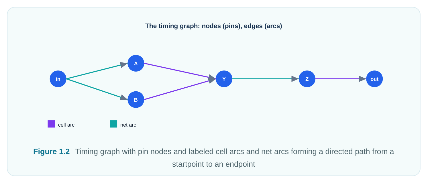
A path is a chain of edges. It runs from a startpoint (a primary input port or a register clock pin) to an endpoint (a register data pin or a primary output port). The tool walks this graph in order. It adds up delay across arcs to build the arrival time at every node. Then it pushes required times backward from the constraints to every node. Subtract one from the other and you get slack. STA computes slack at every pin, not just at endpoints. That is what lets it point you to the exact spot where margin is being lost. For plain logic the graph has no loops. Feedback is cut at register boundaries. So this propagation is a clean, fast, predictable graph walk. That loop-free, pattern-free graph is exactly why STA scales where simulation cannot. One more refinement is worth knowing early. Arrival times are not single numbers. They come in pairs — a latest (max) and an earliest (min). Each pair also carries a transition time (slew, how sharply the signal switches). Slew matters because cell-arc delay depends on it. A slow, lazy edge into a gate makes more delay than a crisp one. Picture pushing a heavy door: a gentle shove takes longer than a firm one. So as STA walks the graph, it carries both delay and slew together. Each arc uses the incoming slew to look up its delay and then puts out a new slew. This pairing of delay and slew is why signal quality and transition limits live inside the same engine as timing, not as a separate add-on.
Where STA Sits in the Design Flow
STA is not a single event at the end of the flow. It is a checkpoint that runs at every major stage of physical build-out. It grows more accurate as more physical reality becomes known. The same engine
and the same constraints get reused each time. What changes is the quality of the delay data feeding the graph.
| Flow Stage | What's Available | STA Accuracy & Purpose |
|---|---|---|
| Post-synthesis | Logical netlist, wireload estimates | Rough, optimistic; sanity-check constraints and architecture |
| Post-placement | Real cell locations, estimated | Better wire estimates; early closure feedback |
routing
Post-CTS (clock tree Real, built clock network Clock skew and latency now real, not ideal
Post-route Extracted parasitics from actual High accuracy; drives final optimization
Signoff Full extraction, all corners, Authoritative; the result you tape out on Early in the flow, before the clock tree exists, the tool uses an ideal clock. That means zero skew and zero insertion delay. Skew is the timing difference between clock arrivals. Insertion delay is how long the clock takes to reach a flip-flop. This lets engineers close the data path before clock realities pile on. After clock tree synthesis, the clock becomes propagated. Now real skew and insertion delay enter the math. By signoff, the analysis uses fully extracted parasitics, every relevant corner, and onchip-variation derating. Derating adds a safety margin for chip-to-chip variation. The result is a verdict you can commit silicon to. The interview takeaway: STA accuracy depends on how much physical truth has been resolved. A clean report at synthesis means very little. A clean report at signoff, across all corners with proper derates, is what actually protects the tape-out. People often ask why the same path can show very different slack across stages. The path did not change. The data feeding the graph did. At synthesis the wire delay was a crude guess. Post-route it is computed from the real metal that was laid down. Before CTS the clock was ideal. After CTS it carries real skew, which can help or hurt a given check. None of this is the tool being flaky. It is the tool faithfully reporting timing against steadily more honest inputs. That is exactly why you re-run STA at each milestone instead of trusting an early result.
The Four Inputs STA Requires
No matter the stage, the timing engine needs four kinds of input. Miss or corrupt any one and the analysis is worthless.
| Input | Format (typical) | Role in the Analysis |
|---|---|---|
| Gate-level | Verilog / structural | Defines the connectivity that becomes the timing graph |
netlist
Timing libraries Liberty-style models Supplies cell delay, setup/hold, slew, and power data
Parasitics Standard parasitic exchange Provides net (wire) R and C for wire delay
Constraints SDC Declares clocks, I/O timing, and exceptions — the The first three describe what the circuit is. The constraints describe what you expect of it. Of the four, constraints are the most error-prone and the most uniquely yours. Libraries and extraction come from your foundry and tool flow. But the constraint set encodes your design intent. That is where most timing-closure mistakes start. Here is a small, portable SDC constraint set. These commands are industry-standard and work across compliant timing tools:
# standard (SDC) — these are industry-standard constraints
# Define an 800 MHz clock (1250 ps period) on the clock port
create_clock -name CLK -period 1250 [get_ports clk]
# Tell STA when inputs arrive, relative to CLK (e.g., 300 ps after the edge)
set_input_delay  -clock CLK 300 [get_ports data_in]
# Tell STA how much time downstream logic needs at the outputs
set_output_delay -clock CLK 250 [get_ports data_out]
# Declare a path that can never be activated, so STA stops flagging it
set_false_path -from [get_ports test_mode] -to [all_registers]
And here is how you might start the analysis and pull a report. These run and report commands are not standardized. Every tool spells them differently. So treat them as generic illustrations of the workflow, not literal syntax:
# illustrative — generic, not tool-specific
read_netlist    top.v               ;# load connectivity
read_library    slow_corner.lib     ;# load timing models for this corner
read_parasitics top.spef            ;# load extracted wire R/C
read_sdc        top.sdc             ;# load the real SDC constraints above
update_timing                       ;# build the graph, propagate arrival/required
# report the worst setup paths to see where slack is tightest
report_timing -delay max -max_paths 10
# report worst hold paths (min-delay checks)
report_timing -delay min -max_paths 10
The pattern to remember: the SDC constraints are real and portable; almost everything that drives the tool or formats a report is vendor-specific. Throughout this handbook we mark commands accordingly so you never confuse the two in an interview.
Interview Q&A
simulation only covers the paths your patterns happen to trigger. It is also far too slow to scale to modern gate counts and corner counts. STA needs no patterns, so it covers every structural path completely. And it runs as a fast graph walk, not an event simulation. You give up functional checking, which STA does not do. In exchange you get guaranteed, complete, fast timing coverage. That is the right trade for sign-off, where functionality is verified separately.
checks what you tell it and trusts its models. Likely culprits: missing or wrong constraints, such as an unconstrained path that was never analyzed, or a false path declared on a real path. Other causes are a library or corner that does not match silicon, missing or wrong parasitics, or too little on-chipvariation derating. A clean STA report is only as trustworthy as the constraints, libraries, extraction, and corners behind it.
graph STA builds from the netlist. Nodes are pins, meaning cell inputs, cell outputs, and ports. Edges are timing arcs. Cell arcs model delay inside a cell, such as input-to-output or clock-to-Q. Net arcs model wire delay from a driver to its loads. STA walks this graph, adding arrival times forward and required times backward, and computes slack at every node.
by other tools, namely functional simulation and logic equivalence checking. It only verifies that signals meet their setup and hold timing. That means the answer, assumed correct, arrives within the clock's timing window. It also cannot tell a logically impossible or multicycle path from a real one unless you declare those exceptions.
Key Takeaways
- STA needs no patterns and is complete. It propagates arrival and required times through a timing graph to check every structural path. It computes slack = required − arrival at each endpoint, with no stimulus.
- It replaced dynamic simulation for sign-off because simulation's coverage depends on patterns and is far too slow, while STA guarantees full coverage at high speed.
- STA checks timing, not function. It assumes function is correct, trusts its library models, and only analyzes what the constraints tell it to.
- The timing graph is the master abstraction: pins are nodes; cell arcs and net arcs are edges; paths run from startpoints to endpoints.
- STA runs at every flow stage — synthesis, placement, CTS, route, signoff — and gets more accurate as physical reality (real clock tree, extracted parasitics, all corners) is resolved.
- It needs four inputs: netlist, timing libraries, parasitics, and constraints. The SDC constraints are real and portable and are where most closure mistakes start; most run and report commands are vendor-specific.
Comments
Leave a Reply