 ChipBuddy
← Home
ChipBuddy
← Home
Multi-Clock Timing & Phase Relationships
Dive)
Most beginner STA (Static Timing Analysis, checking timing without running the chip) examples assume one clock. The flop that sends data and the flop that catches it share the same clock. Real chips are not so simple. A modern SoC (System on Chip, one chip with many parts) has many clocks. There is a fast core clock. There is a slower bus clock. There are divided clocks for peripherals. There are phase-shifted clocks for memory. Some clocks share nothing but power. A path runs from one flop to another flop. When that path crosses from one clock to another, a hard question appears. Which edge of the sending clock races which edge of the catching clock? An edge is a clock's rising tick. This chapter explains how STA answers that for related clocks. Related clocks share a common timebase. We build the math from scratch. We work the classic 4 ns to 6 ns case. We handle samespeed clocks that are shifted in phase. We reason about which directions are truly hard. Truly unrelated clocks are the next chapter. Here the relationship is real and the constraint matters.
17.1 Why a Single Edge Pair Is Not Enough
In a same-clock setup check, life is easy. The launch edge and the capture edge are always one period apart. So the setup budget is just the period T . With two clocks, that breaks. Each clock has its own period or phase. The launch flop fires on clock A edges. The capture flop samples on clock B edges. Over time the two edge streams drift past each other. The smallest positive gap from a launch edge to the next capture edge sets the setup rule. That gap can be much smaller than either period. STA handles this by expanding both clock waveforms. It draws them over a window long enough to show every alignment. Then it lists edge pairs. The window length is the common period. The common period is the LCM (Least Common Multiple, the smallest number both periods divide into) of the two periods. Inside one common period the pattern repeats. So one window is enough.
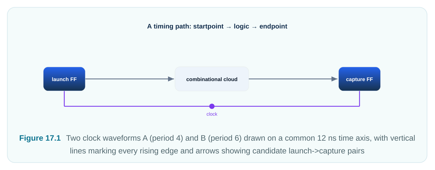
The engine then uses two rules:
- Setup (max) analysis: pick the launch and capture pair with the smallest positive gap (launch edge to capture edge). This is the tightest deadline. It is the worst case.
- Hold (min) analysis: pick the pair where fresh data could overwrite data just captured. These are the edges closest to colliding in the hold direction. The setup pair and the hold pair are usually not the same. This trips up many people in interviews.
17.2 The Common-Period Expansion, Step by Step
Let clock A have period Ta . Let clock B have period Tb . Both start a rising edge at t = 0. The steps:
- 1. Find the common period
Tc = LCM(Ta, Tb). - 2. List all A rising edges in
[0, Tc]: 0, Ta, 2·Ta, … - 3. List all B rising edges in
[0, Tc]: 0, Tb, 2·Tb, … - 4. For setup, take each A launch edge. Find the nearest B capture edge strictly after it. The smallest
such gap is the setup capture relationship.
- 5. For hold, use the capture edge picked for setup. Pair it with the launch edge one cycle later, plus
nearby pairs. Keep the smallest.
| Term | Meaning |
|---|---|
| Launch edge | The clock edge at the source flop that releases data |
| Capture edge | The clock edge at the destination flop that samples data |
| Setup relationship | Smallest positive (capture − launch) over the common period |
| Hold relationship | Tightest (capture − launch) that must stay non-negative for safe data |
| Common period (Tc) | LCM of the two periods; the size of the expansion window |
The setup relationship is the budget. The combinational logic plus setup time must fit inside it. A small setup relationship means a tight constraint.
17.3 Worked Example 1 — 4 ns ↔ 6 ns
Take clock A at 4 ns (250 MHz). It launches to clock B at 6 ns (about 166.7 MHz). Both edges line up at t = 0.
Tc = LCM(4, 6) = 12 ns.A (launch) rising edges in [0, 12]: 0, 4, 8, 12 B (capture) rising edges in [0, 12]: 0, 6, 12 For each launch edge, find the nearest later capture edge:
| Launch edge (A) | Next capture edge (B) | Setup separation |
|---|---|---|
| 0 | 6 | 6 ns |
| 4 | 6 | 2 ns |
| 8 | 12 | 4 ns |
The worst gap is 2 ns. It comes from launch at t = 4 to capture at t = 6. Neither clock period is below 4 ns. Yet the effective setup budget is only 2 ns. The data path plus setup time must fit in 2 ns. This is why multi-clock paths are dangerous. The LCM window can be tighter than either clock alone. Setup check (numeric): suppose the data path delay (clk→Q + logic + net) is 1.20 ns. Destination setup is 0.30 ns. Setup uncertainty is 0.20 ns.
# illustrative — generic, not tool-specific
Required time = 2.00 (relationship) - 0.30 (setup) - 0.20 (uncertainty) = 1.50 ns
Arrival time  = 1.20 ns
Slack = Required - Arrival = 1.50 - 1.20 = +0.30 ns   (PASS)
Hold check: hold uses the worst near-collision pair. STA searches all adjacent pairs. The tightest case is launch at t = 0 against capture at t = 0. Both sit at zero. That gives a 0 ns hold relationship. This is the classic worst case. Hold passes only if the real data path delay beats the hold time plus hold uncertainty.
# illustrative — generic, not tool-specific
Hold required = 0 (relationship) + 0.12 (hold time) + 0.06 (uncertainty) = 0.18 ns
Earliest data arrival (min path) = 0.27 ns
Hold slack = Arrival - Required = 0.27 - 0.18 = +0.09 ns   (PASS)
The lesson is simple. The setup pair (4 → 6) and the hold pair (0 → 0) differ. The tool reports them on their own.
17.4 Integer, Rational, and Non-Integer Ratios
The nature of the constraint depends on the ratio of the two periods.
| Relationship | Example periods | Common period | Typical effective setup |
|---|---|---|---|
| Integer (harmonic) | 2 ns & 4 ns | 4 ns | Equal to faster period (clean) |
| Simple rational | 4 ns & 6 ns | 12 ns | Can be a small fraction (2 ns here) |
| Awkward rational | 5 ns & 7 ns | 35 ns | Often very tight (1 ns or less) |
| Near-integer non-harmonic | 10 ns & 10.1 ns | huge / impractical | Beat frequency, extremely tight |
Integer (harmonic) ratios are the kindest. Say A is exactly twice the frequency of B (Ta = 2, Tb = 4). Edges line up cleanly. Every B edge sits on an A edge. The setup window equals the faster period. No tight window is created. Simple rational ratios give a finite common period. Think 2:3 for 4 ns and 6 ns. It is manageable. But it can still be tight, as we saw. Awkward rationals are the trap. Periods of 5 ns and 7 ns give an LCM of 35 ns. Somewhere in that window a launch edge lands just before a capture edge. The setup window shrinks to 1 ns or less. The tool enforces it. The path fails. The designer is puzzled, since "neither clock is that fast." Non-integer ratios like 10 ns and 10.1 ns have a huge or undefined LCM. STA caps the expansion at a set number of cycles. It reports the tightest pair found. Such pairs often mean the clocks should be treated as asynchronous. If the relationship is not physical, the fix is to declare them so (next chapter). Do not chase an impossible 0.3 ns path. Rule of thumb: the messier the ratio, the tighter and less physical the constraint. Always check if a hard multi-clock path is truly synchronous before spending effort on it.
17.5 Same-Frequency, Phase-Shifted Clocks
A common case is two clocks of the same period with a planned phase offset. Think of a 0° clock and a 90° (quarter-period) shifted clock. These show up in quadrature interfaces. Let both clocks have period T = 4 ns . Clock A launches at 0, 4, 8, … Clock B is shifted by +90° = 1 ns. Its edges fall at 1, 5, 9, …
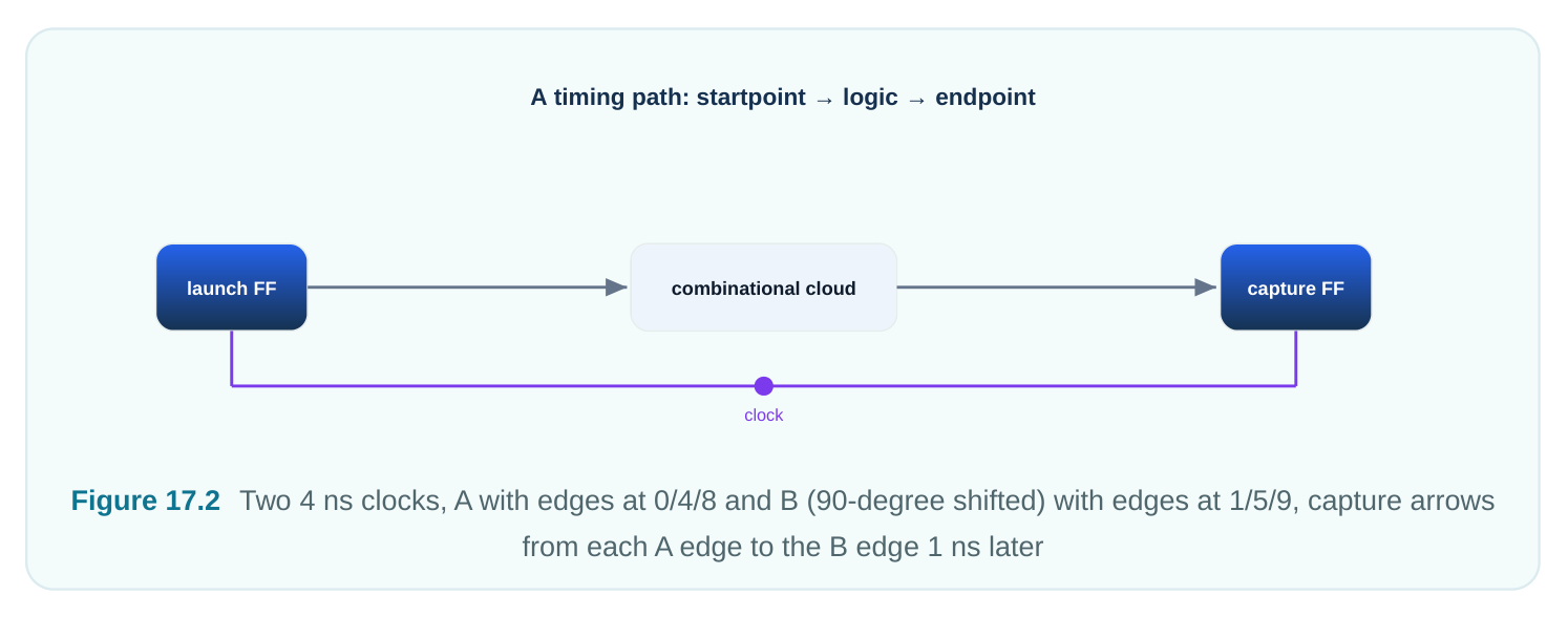
Setup relationship: launch at 0 to the next B edge at 1 gives 1 ns. The phase shift becomes the budget. A 90° lead on the capture clock leaves only a quarter period for data.
| Capture phase | Capture edge after launch@0 | Setup window |
|---|---|---|
| 0° (aligned) | 4 | 4 ns (full period) |
| +90° (early) | 1 | 1 ns (tight) |
| +180° | 2 | 2 ns |
| −90° (late, i.e. 270°) | 3 | 3 ns (relaxed setup) |
Notice the symmetry. A capture clock that is phase-advanced tightens setup but relaxes hold. A capture clock that is phase-delayed relaxes setup but tightens hold. With +90°, hold becomes the easy check. The next launch at t = 4 is far from the capture at t = 1. Phase trades one check for the other. You rarely get both free.
# standard (SDC)
create_clock -name clkA -period 4.0 [get_ports clkA]
create_clock -name clkB -period 4.0 [get_ports clkB]
# express the 90-degree (1 ns) phase shift via the waveform
create_clock -name clkB -period 4.0 -waveform {1.0 3.0} [get_ports clkB]
The -waveform {rise fall} form tells the engine the phase shift. The rising edge of clkB is set at 1.0 ns, not 0.0 ns. STA then carries that into every launch and capture relationship on its own.
17.6 Slow-to-Fast vs Fast-to-Slow: Which Is Harder?
Both directions are tricky. They fail in different ways. Fast launch → slow capture (e.g., 4 ns → 6 ns): This is the classic setup squeeze. The fast clock gives dense launch edges. One lands just before a sparse capture edge. That creates the tight 2 ns window we computed. Setup is the main risk. Slow launch → fast capture (e.g., 6 ns → 4 ns): Here the capture clock is dense. A capture edge often comes soon after a launch edge. That squeezes setup. It also makes hold nasty. The next capture edge arrives fast. The launched data must not still be in flight at the previous capture edge. Hold violations grow. Dominant
Direction Why
| Fast → slow | Setup | Dense launch edge lands just before sparse capture edge |
|---|---|---|
| Slow → fast | Setup + hold | Dense capture edges create tight deadlines and easy hold |
collisions
Same freq, capture Setup Reduced window equal to phase lead
Same freq, capture Hold Next launch races the delayed capture edge In general, slow-to-fast is the harder one to close. It stresses setup and hold at once. The dense capture clock leaves no room to fix hold by padding delay without breaking setup. Many designs add pipeline stages. Others treat such crossings as asynchronous rather than fight both constraints.
17.7 When Related-Clock Timing Is Real — and When It Is Not
The expansion above is valid only if the two clocks are physically phase-coherent. That means they share one source and hold a fixed, known phase at the registers. This is true when:
- Both clocks come from the same PLL or oscillator through fixed dividers.
- The skew between them is bounded and measured.
- The launch and capture edges truly happen at the times the SDC waveforms describe. It is not true when the clocks come from separate sources. It is not true when the phase between them is unknown. It is not true when the LCM is huge. In those cases the alignments STA enumerates are fictional. The reported "worst" 0.3 ns path is meaningless. Forcing closure wastes effort. The right treatment for unrelated clocks is to declare them so. This removes the false checks. You then rely on proper clock-domain-crossing (CDC) synchronizers. That declaration and those structures are
the next chapter. For now the rule is clear. Before optimizing a hard multi-clock path, prove the relationship is real.
17.8 Constraining Multi-Clock Interactions
By default the engine times every path between every pair of clocks. You shape this with clock groups and exceptions. Clock groups tell the engine how clocks relate. Two important kinds:
# standard (SDC)
# Declare two clocks as asynchronous: do NOT time paths between them
set_clock_groups -asynchronous \
-group {clk_core} \
-group {clk_periph}
# Declare clocks as physically exclusive (never active at the same time,
# e.g. two muxed sources on one tree): also no cross-timing
set_clock_groups -physically_exclusive \
-group {clk_pll} \
-group {clk_test}
For clocks you do want timed together, just define them with the right periods and waveforms. Let the expansion run. If one crossing needs a looser deadline, a multicycle path is the tool:
# standard (SDC)
# Give the 4ns -> 6ns crossing two capture cycles instead of one
set_multicycle_path 2 -setup \
-from [get_clocks clkA] -to [get_clocks clkB]
set_multicycle_path 1 -hold \
-from [get_clocks clkA] -to [get_clocks clkB]
Be careful with the hold multiplier. A setup multicycle without a matching hold change makes a false extra-cycle hold rule. The tool will then try and fail to meet it. Per-clock uncertainty lets you model jitter and skew per domain and per check direction:
# standard (SDC)
# Tighter uncertainty on the high-speed clock, looser on the slow bus clock
set_clock_uncertainty -setup 0.12 [get_clocks clkA]
set_clock_uncertainty -hold  0.05 [get_clocks clkA]
set_clock_uncertainty -setup 0.20 [get_clocks clkB]
# Inter-clock uncertainty: extra margin specifically on the crossing
set_clock_uncertainty -setup 0.18 -from [get_clocks clkA] -to [get_clocks clkB]
The -from/-to form is very useful for multi-clock work. Crossings often carry more uncertainty than paths inside one domain. The two clock trees may share little structure. So their skews do not cancel.
| Construct | Purpose | Effect on cross-clock timing |
|---|---|---|
| set_clock_groups -asynchronous | Declare unrelated clocks | Removes all paths between |
groups
set_clock_groups - Mutually-exclusive Removes paths; clocks never co-| physically_exclusive | sources | active |
|---|---|---|
| set_multicycle_path | Relax a real but slow crossing | Widens the capture window by N cycles |
| set_clock_uncertainty -from -to | Model inter-domain skew/jitter | Adds margin only on the crossing |
17.9 Worked Example 2 — Phase-Shifted Capture Slack
Now mix the phase idea with real numbers. Clock A and clock B are both 4 ns. B is the 90° (1 ns) advanced capture clock from Section 17.5. That gives a 1 ns setup relationship. Data path: clk→Q = 0.35 ns, logic = 0.50 ns, net delay = 0.10 ns. Arrival = 0.95 ns. Destination setup = 0.15 ns. Inter-clock setup uncertainty = 0.10 ns.
# illustrative — generic, not tool-specific
Required = 1.00 (relationship) - 0.15 (setup) - 0.10 (uncertainty) = 0.75 ns
Arrival  = 0.95 ns
Setup slack = 0.75 - 0.95 = -0.20 ns   (FAIL)
The 90° shift left only 1 ns. After setup and uncertainty the path misses by 200 ps. Options: speed up the data path (less logic depth), reduce the phase advance, retime the capture clock to a softer phase, or apply a multicycle exception if the path is not needed every cycle. Compare with the aligned (0°) case. There the relationship would be the full 4 ns. The same path would pass with huge margin (about +2.80 ns). Phase, not period, killed this path. That is the key intuition of this chapter.
17.10 Interview Q&A
pattern of edge alignments repeats exactly every LCM(Ta, Tb). Checking one window is both needed and enough. It finds the worst launch and capture pair. Beyond it, alignments just repeat.
window, and which edges set it? The LCM is 12 ns. Launch edges 0/4/8 race capture edges 0/6/12. The tightest is launch at 4 to capture at 6 = 2 ns. So the logic plus setup must fit in 2 ns. Neither clock period is that small.
error. Setup uses the smallest positive launch-to-capture gap. Hold uses the pair where fresh data could overwrite just-sampled data. In the 4 ns/6 ns case, setup is 4→6. The worst hold pair is 0→0.
Somewhere in that long window a launch edge lands a hair before a capture edge. That gives a setup window of about 1 ns or less. The tool sees it as real. It often is not physical. That hints the clocks may belong in separate, asynchronous groups.
capture clock advanced by 90° shrinks setup to a quarter period (1 ns for a 4 ns clock). It relaxes hold, since the next launch is far from the early capture edge. Phase shifts trade setup against hold. A delayed capture clock does the opposite.
phase-coherent. That means separate sources, unbounded phase, or a huge LCM. The alignments are then fictional. Declare the clocks asynchronous with set_clock_groups -asynchronous . Synchronize the crossing with proper CDC logic. Do not optimize a meaningless constraint.
Key Takeaways
- Between two related clocks, STA expands both waveforms over the common period (LCM of the two periods) and lists edge pairs to find the worst setup and worst hold.
- The setup window is the smallest positive launch-to-capture gap. It can be far tighter than either period. 4 ns ↔ 6 ns gives only a 2 ns budget.
- Setup-critical and hold-critical edge pairs usually differ. Report and reason about them on their own.
- Period ratio matters a lot. Harmonic (integer) ratios are clean. Simple rationals are manageable. Awkward rationals (5:7) and near-equal periods give very tight, often unphysical windows.
- For same-frequency phase-shifted clocks, the phase offset becomes the budget. A 90° advance leaves a quarter period for setup. Express phase with
-waveform. - Slow-to-fast crossings are generally hardest. They stress setup and hold at once. Fast-to-slow mainly squeezes setup.
- Before optimizing a hard crossing, verify the relationship is real. If not, declare the clocks asynchronous and use CDC. That is the next chapter.
- Shape cross-clock timing with
set_clock_groups,set_multicycle_path(with matched hold), and per-crossingset_clock_uncertainty -from -to.
Comments
Leave a Reply