 ChipBuddy
← Home
ChipBuddy
← Home
Hierarchical STA & Timing Models
Why Full-Chip Flat STA Eventually Breaks Down
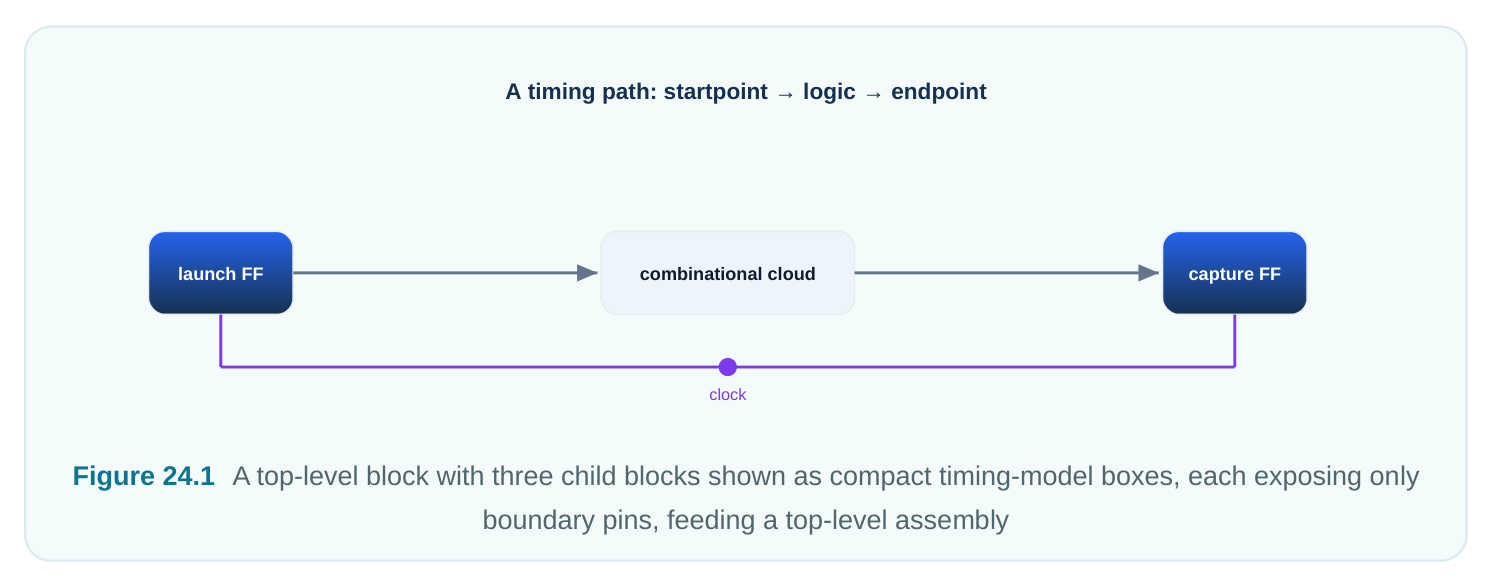
A small block can be timed flat. "Flat" means every cell and every net is checked at once. This works for a small design. A full SoC (system-on-chip, one whole chip) cannot be timed this way. It has hundreds of millions of instances (cell copies). Memory and runtime explode. Also, no single engineer owns the whole netlist (the gate-level description of the chip). The fix is hierarchical static timing analysis. Here each block is timed on its own. Then the top level sees a small timing model (a compact stand-in for the block) instead of all its gates. Think of it like a phone book entry. You get the key facts, not the whole person. This chapter covers the model types, their use, and the traps.
The Two Families of Block Timing Models
There are two main ways to abstract (simplify into a stand-in) a block. The difference matters in interviews. A boundary timing model keeps only what is visible at the pins. This means the arcs (timing paths) from inputs to outputs. It also keeps the setup and hold needs at input registers. It keeps clock-tooutput delays too. And it keeps input/output capacitance and drive strength. The inside logic is thrown away. The block becomes a black box. It is small and fast. But it hides the internal paths. An interface logic model is different. It keeps the real gates on paths that touch the boundary. That means the first and last levels of logic, plus the registers they connect to. It removes only the deep internal logic that the outside cannot reach. It is bigger than a boundary model. But it is more accurate. Real cells time the interface, not abstract arcs. It also handles tricky cases better, like on-chip variation (small timing differences across the chip).
| Model type | What it keeps | Size | Accuracy | Good when |
|---|---|---|---|---|
| Boundary (extracted) | boundary arcs + model | smallest constraints only | good if context- correct | stable interfaces, max compression |
| Interface logic model | real interface gates + | medium | higher registers | OCV-sensitive interfaces, reuse |
| Full block (flat) | everything | largest | exact | small blocks, final checks |
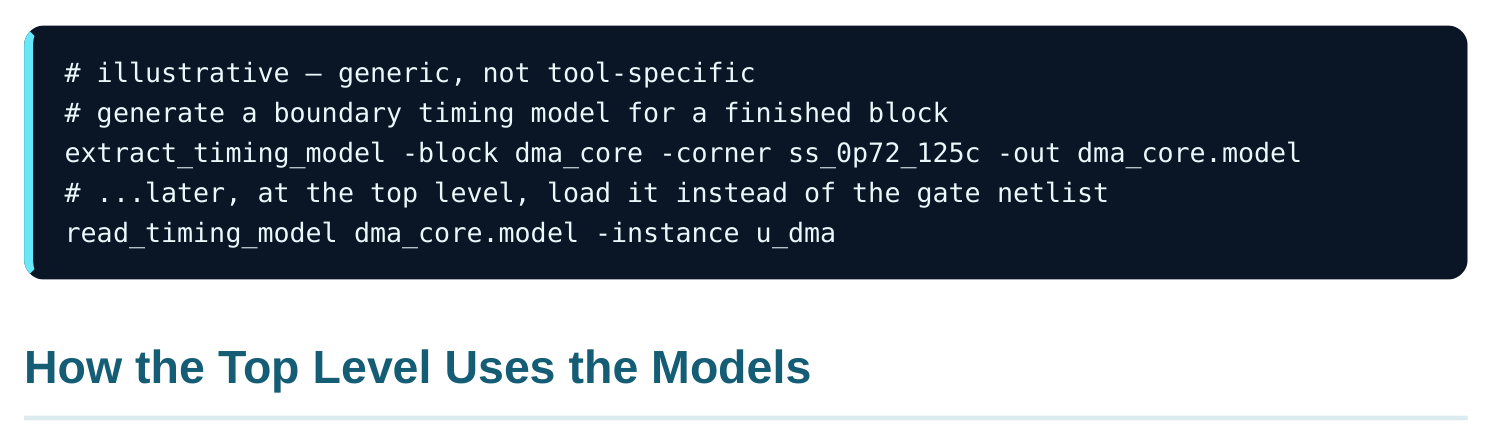
At the top level, the engine joins the block models together. It adds the top-level glue logic and clocks. Each model gives three things.
- Input setup/hold needs. The top level must meet these at the block's input pins.
- Clock-to-output arcs. These drive top-level paths going downstream.
- Clock definitions and latency at the boundary. This lets the top see the block's clocking right. The key rule is context consistency. A model is only valid for the corner, mode, and boundary conditions it was made with. (A corner is one set of voltage, temperature, and process. A mode is one operating state.) Say the block was built at one corner. Then it is used at the top in another corner. The
numbers mean nothing. So model the block at every corner and mode the top will use. Then bind the right model in each run.
| Boundary item in a model | Used at top level for |
|---|---|
| Input setup/hold | constraining top→block paths |
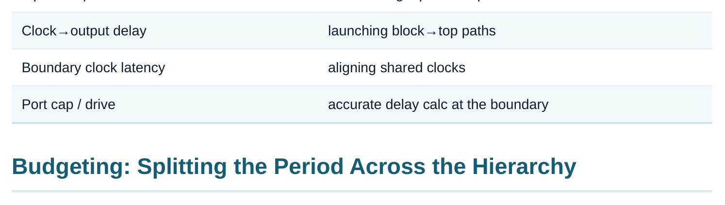
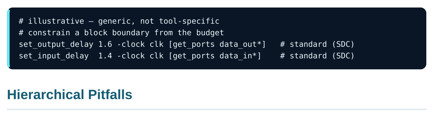
Top-level timing is unknown before blocks are built. So each interface gets a budget. A budget is a share of the clock period. It splits between the block side and the top side of each boundary path. The block is then built to meet its budget. The top is built to meet the rest. Get the split wrong and trouble follows. Blocks may pass alone but fail when joined. Or they get over-constrained for no reason. Budgeting is iterative. You start with estimates. You refine them once real models exist.
Worked example — boundary budget
A path crosses a block boundary. It is register-to-register. The period is 2.5 ns. Split it like this. Give 0.9 ns to logic inside block A. This is A's output delay budget. Give 0.5 ns to top-level glue and wires. Give 1.1 ns to logic inside block B. This is B's input delay budget. The three add to 2.5 ns. Now constrain block A. Its output delay is 0.5 + 1.1 = 1.6 ns. Constrain block B too. Its input delay is 0.9 + 0.5 = 1.4 ns. Say A really needs 1.2 ns and B really needs 0.7 ns. The total is 1.9 ns. That still fits 2.5 ns. But the per-side split was off. A fails alone while B has slack. Refinement moves the split.
Hierarchical timing has failure modes that flat timing never has.
- Context mismatch. The model was made under different boundary loads or clocks than the top uses. The result is silent inaccuracy.
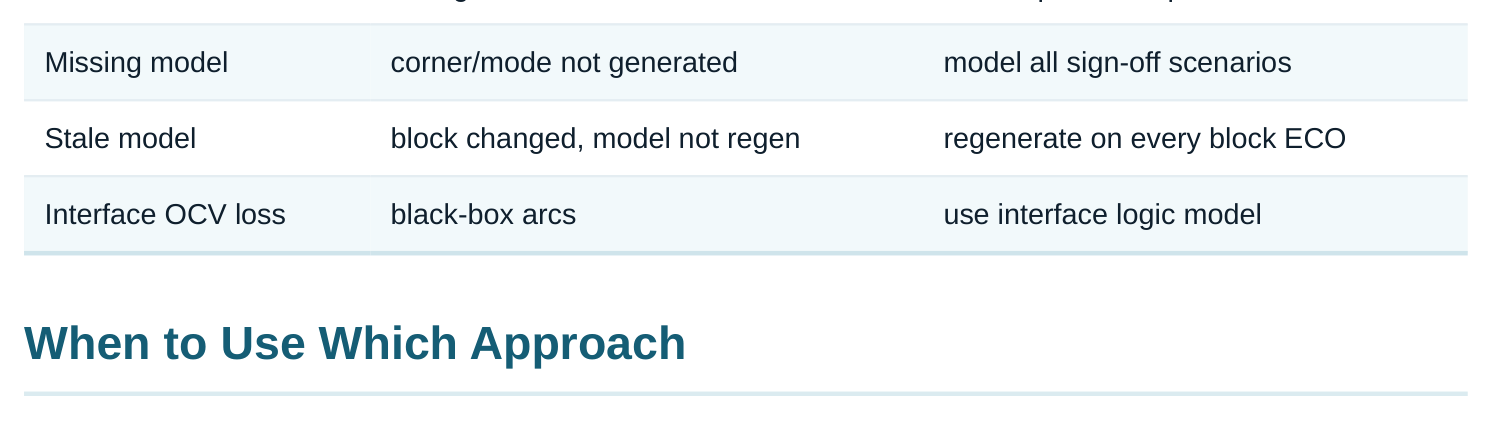
- Missing corner/mode model. The top needs a corner the block was never modelled at.
- Lost internal margin. A pure boundary model can hide a path that barely passes inside. If the block changes, you must redo the model. Else the top sees stale timing.
- OCV at the interface. A black-box arc cannot derate by path depth. Real interface gates can. (Derating means adding margin for variation.) So prefer interface logic models on variation- sensitive boundaries.
- Clock reconvergence across the boundary. Shared clocks must be described the same way. Else CPPR (common path pessimism removal) is mishandled at the top. Pitfall Cause Mitigation Context mismatch wrong extraction conditions extract per real top context
Flat timing stays the gold standard. Use it for small blocks and final confidence runs. Hierarchical timing with boundary models gives the most compression. Use it for large, stable blocks. Interface logic models sit in the middle. Use them when interface accuracy matters, especially under variation. Most large projects mix all three. Leaf blocks stay flat. Mid-level blocks become interface logic models. The very top is built from models. Periodic flat "stitch" checks catch any modelling errors.
Interview Q&A
runtime will not allow it. Also, ownership is split across teams. Each block is timed once. It is then shown by a small timing model at the top. This makes full-chip timing doable.
That means arcs, setup/hold, and clock-to-out. It drops the inside gates. It is smallest and fastest. An interface logic model keeps the real gates on boundary-touching paths. It drops only deep internal logic. It is larger but more accurate. It is better for OCV at the interface.
the corner, mode, and boundary conditions it was made with. Use it in another scenario and the numbers are wrong. So model the block at every sign-off corner and mode the top uses.
blocks exist. The split gives a block-side share and a top-side share. These become input and output delay constraints. The first splits are guesses. Once real timing is known, you refine them. Then blocks that pass alone also pass when joined.
path depth through real cells. A black-box arc has no internal depth to derate. So interface variation can be modelled wrong. Keeping real interface gates restores correct depth-based derating.
Key Takeaways
- Hierarchical STA replaces each block with a small timing model so full-chip timing stays doable.
- Boundary models are smallest. Interface logic models keep real boundary gates for higher accuracy, especially under OCV. Flat is exact but heavy.
- Models are context-specific. Extract one per corner, mode, and boundary condition. Regenerate after block changes.
- Interface budgeting splits each boundary path's period into block and top shares. Refine it so isolation results match assembly.
- Most flows mix flat, interface-logic, and boundary models, with periodic flat checks to catch modelling errors.
Comments
Leave a Reply