 ChipBuddy
← Home
ChipBuddy
← Home
On-Chip Variation (OCV/AOCV/POCV) & CPPR
Reconvergence Pessimism
We sign off a design at a PVT corner (a fixed mix of process, voltage, and temperature). That corner assumes every transistor on the chip behaves the same way. This is handy but not true. Two gates sitting close together are never identical. They differ in threshold voltage, channel length, and oxide thickness. The corner only captures how the whole wafer shifts. It says nothing about the small scatter between neighbors. This chapter shows how STA handles that gap. The launch path and the capture path do not see the same silicon. We model that difference. Then we remove the extra pessimism we added by accident.
Why One Corner Is Too Crude
A setup check compares two times. One is when launch data arrives at the capture flop. The other is when the capture clock edge arrives. Both are found by walking through real cells. If we delay both with the same corner, we claim launch cells and capture cells are equally fast. That is wrong. Variation has two parts.
- Global / systematic variation — the whole chip shifts as one. The wafer ran fast, or the chip is hot. A corner models this. It cancels out, because launch and capture shift together.
- Local / random variation — each device drifts on its own. This does not cancel. Launch cells may be slightly slow while capture clock cells are slightly fast. That eats your setup margin. Local variation forces us past one corner. STA must show the worst likely speed gap between launch and capture. The absolute speed of the chip is not enough.
Basic OCV: Opposite Derates
The first answer is classic On-Chip Variation (OCV). The idea is simple. We push launch and capture in opposite directions. This models their worst spread. For a setup check, we want launch data late and the capture clock early. So we slow the launch path with a late derate above 1.0. We speed the capture clock with an early derate below 1.0. For a hold check we flip it. We speed the launch data and slow the capture clock.
# standard (SDC)
# Late paths run up to 7% slower, early paths up to 7% faster
set_timing_derate -late  1.07 -cell_delay -net_delay
set_timing_derate -early 0.93 -cell_delay -net_delay
The tool picks which derate goes on which path. It always picks the pessimistic way. The good part is that it is simple. The bad part is too much pessimism. A flat 7% on a 30-stage path assumes all 30 cells turn slow at once. That almost never happens. So OCV over-derates long paths. It can chase failures that never occur in real silicon.
Advanced / Parametric OCV (AOCV)
Advanced OCV cuts the pessimism. It uses one key fact. Random variation averages out over more stages. Say each cell delay has an independent spread of one sigma (a measure of how much delay varies). A path of N cells has a relative spread that shrinks near 1/sqrt(N). A short two-stage path can swing a lot. A fifty-stage path cannot. The highs and lows cancel. AOCV uses derate tables. The tables are indexed by two things.
- Logic depth — how many stages the path passes through. More depth means a smaller derate.
- Physical distance — how far the path spreads across the chip. Slow gradients (Vt or heat slopes) grow with distance. So a wider reach earns a bigger systematic part. The tool reads a derate from a 2-D table. It uses the path's real depth and span. It does not slam one number onto everything.
# illustrative — generic, not tool-specific# Load a depth/distance-indexed derate table for a library groupread_aocv_table ./derate/stdcell_aocv.tblset_aocv_analysis_mode -enable trueAOCV wins back a good slice of OCV pessimism on deep paths. It stays safe on short ones. Its weak point is this. It still gives one number per path. It threw away the full spread and kept only a bounded multiplier.
Statistical / Parametric OCV (POCV / SOCV)
POCV (also sold as SOCV) goes deeper. It keeps the full spread. Each cell delay is a random variable. It has a mean and a sigma. The sigma usually scales with the cell's nominal delay. It comes per library, through a coefficient or an LVF table. Path delay becomes a sum of independent random variables. The means add straight up. The variances add too. So sigmas combine in quadrature: sigma_path = sqrt(sum of sigma_i squared). The tool reports slack at a chosen confidence. Often this is plus or minus 3 sigma. Variances add, not sigmas. So a long path's total sigma stays small next to its mean. POCV is less pessimistic and more accurate than flat OCV. It is AOCV's averaging idea done with real math, not lookup tables.
# illustrative — generic, not tool-specific
# Switch the engine to parametric (statistical) variation
set_pocv_analysis  -enable true -sigma 3.0
read_lvf_data  ./derate/stdcell_lvf.lib   ;# per-cell mean + sigma
POCV needs richer library data. It needs variation data per cell and per arc. In return it gives tighter, defensible slacks. It is the modern default for advanced nodes. There the gap between OCV pessimism and reality costs too much to ignore.
VARIATION MODELS COMPARED
| Model | How it derates delay | Relative pessimism |
|---|---|---|
| Single | One factor for whole die; launch/capture | Misses local variation entirely (optimistic on |
| corner | identical | relative skew) |
| Basic OCV | Flat opposite derate, launch vs capture | High — assumes every cell deviates |
together
| AOCV | Scalar derate from depth/distance table | Medium — credits averaging over stages | |
|---|---|---|---|
| POCV / | Per-cell mean + sigma, RSS-combined, SOCV | Low — statistically accurate reported at N-sigma | |
| Aspect | OCV | AOCV | POCV |
| Granularity | Constant per design | Per path (depth, distance) | Per cell (distribution) |
| Library data needed | Derate factor | Depth/distance tables | Mean + sigma (LVF) |
| Path-length awareness | None | Via lookup table | Inherent (RSS) |
| Accuracy | Crude | Better | Best |
| Runtime cost | Lowest | Moderate | Highest |
Clock Reconvergence Pessimism (CRPR / CPPR)
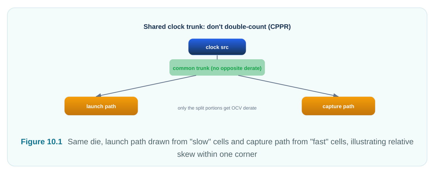
Here is the subtle part. It matters a lot. In every flop-to-flop check, the launch clock and the capture clock share part of their route. Both start at the clock source. Both run together through the clock tree. Then they split off toward their own flops.
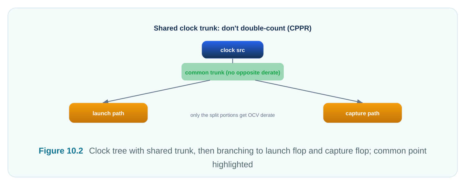
Now we apply opposite OCV derates. We slow the launch clock and speed the capture clock, or the reverse. But the shared part is the same wire and the same buffers. One set of devices cannot be fast for one path and slow for the other at the same time. Applying opposite derates there counts a gap
that cannot exist. This fake penalty is clock reconvergence pessimism (CRP). The fix is CRPR / CPPR (clock reconvergence path pessimism removal). The flow is simple.
- 1. Find the common point. It is the last node both clock paths share.
- 2. Measure how much opposite derate (or sigma) was applied to that shared part.
- 3. Give it back to the check. The shared devices act the same for both edges.
CPPR removal is not a tiny tweak. On deep clock trees it can win back hundreds of picoseconds. It often flips a reported violation into a passing path. It must always be on for real OCV/AOCV/POCV sign-off. Leave it off and you get large fake failures.
# illustrative — generic, not tool-specific
# Enable clock reconvergence pessimism removal
set_timing_analysis  -crpr_removal true
report_timing -crosstalk_delta -crpr ;# show the credit per path| Concept | Without CPPR | With CPPR |
|---|---|---|
| Shared clock trunk | Derated oppositely for launch/capture | Recognized as common; opposite derate |
removed
Reported Inflated (double-counted) Realistic
| Effect on slack | Artificially negative | Recovered, often large |
|---|---|---|
| Sign-off validity | Unsafe (over-pessimistic, wasted closure | Correct |
effort) A handy check for interviews. CPPR is the credit you give back. The clock source and shared tree feed both edges from the same hardware. So their common-path variation is perfectly correlated, not opposed.
Graph-Based vs Path-Based Recovery
The variation handling above is usually run first in graph-based analysis (GBA). GBA pushes one worst-case arrival per node through the timing graph. It is fast and complete. But it is pessimistic. It assumes worst-case derate and slew can all happen on the same path. Path-based analysis (PBA) revisits the specific failing paths. It recomputes them with the actual slews, the actual depth, and properly correlated derates. It drops the worst-case-everything view that GBA carries. For OCV, it tightens the per-stage derate to the real path. For POCV, it recomputes the true sigma along the real arc order. PBA almost always wins back slack GBA left behind. So the usual flow runs GBA broadly. Then it runs PBA on the leftover violators before calling a path a real failure. (PBA has its own chapter. Here, see it as the per-path refinement of these same models.)
Putting It Together
A real modern setup/hold sign-off stacks these steps. Pick a variation model. Use OCV for mature nodes. Use AOCV or POCV for advanced ones. Apply opposite launch/capture derating. Always remove clock reconvergence pessimism. Run graph-based first. Recover the rest with path-based analysis. Each layer trades runtime for accuracy. Each one strips off a slice of pessimism the layer below could not tell apart from real risk.
Interview Q&A
corner does? A global corner shifts both paths the same way. So a setup check sees the same relative timing, and it cancels. OCV applies opposite derates on purpose. It puts late on one path and early on the other. It does this because it models local random variation. Local variation does not move both paths together. The whole point is to expose the worst relative gap. So by design it does not cancel.
averages out over more stages. The relative spread of a sum of N independent delays shrinks near 1/ sqrt(N). Basic OCV ignores this. It applies the same flat derate at any depth. That assumes all N stages drift the same way at once. AOCV's depth-indexed table credits the averaging. So deep paths get a smaller derate.
opposite derate that OCV put on the shared clock-tree part. The launch and capture clock paths share that part. Those buffers and wires are the same hardware feeding both edges. They cannot be fast for one and slow for the other. Applying opposite derate there counts an impossible gap. Ignoring CPPR inflates pessimism, often by hundreds of picoseconds. That makes fake violations and wastes closure effort on paths that pass in silicon.
AOCV reduces variation to one scalar derate per path from a table. POCV keeps each cell delay as a spread (mean plus sigma). It adds the means straight up. It combines the sigmas in quadrature (RSS). Then it reports slack at a chosen confidence, such as 3 sigma. Variances add, not sigmas. So long paths get a smaller total spread. That matches the real physics of independent random variation. So POCV is tighter and more defensible than AOCV's table scalar.
Key Takeaways
- A single corner models global die shift but not local random variation between neighbors. Launch and capture paths do not see the same silicon.
- Basic OCV applies opposite derates to launch and capture to expose worst-case skew. It is simple but very pessimistic, since it assumes every cell drifts together.
- AOCV indexes derate by logic depth and physical distance. It credits the fact that random variation averages out over more stages.
- POCV / SOCV models each cell delay as a mean plus sigma. It combines variances in quadrature and reports slack at N-sigma. It is the most accurate and least pessimistic model.
- Clock reconvergence pessimism removal (CRPR / CPPR) gives back the opposite derate wrongly applied to the shared clock-tree part. It is essential, often large, and must always be on.
- Graph-based analysis applies these models fast but pessimistically. Path-based analysis wins back slack on real failing paths using actual slews, depth, and correlated derates.
Comments
Leave a Reply