 ChipBuddy
← Home
ChipBuddy
← Home
Clocks: Latency, Uncertainty, Skew & Jitter
Chapter 6 — Clocks: Definition, Latency, Uncertainty, Skew &
Jitter
Every timing check rests on a clock. The clock tells the analyzer two things. It says when a launching flip-flop (a 1-bit memory cell) sends data. It says when a capturing flip-flop reads that data. If the clock model is wrong, every later number is wrong too. Worse, it fails silently. So good engineers fix the clock model first. They get the definitions, latencies, and uncertainty right. Only then do they look at slack (the spare time on a path). This chapter builds the clock model step by step. We start with how a clock is described. We then cover where its delay comes from. Next we model a real clock's flaws with one budget knob. Finally we replace that knob with physical reality: skew and jitter.
6.1 Defining a Clock
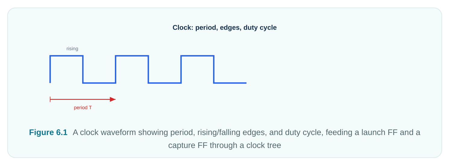
A clock definition gives the analyzer three things. It gives a period, a waveform, and a source. The source is the pin or port where the clock enters or starts. The period is the time between two matching edges. Usually it is rising edge to rising edge. The waveform says where the edges sit inside one period. A 50% duty-cycle clock rises at time 0. It falls at the half-period. Duty cycle means the fraction of the period the clock is high. A non-50% clock just moves the falling edge. A 70% high-time clock on a 10 ns period rises at 0 and falls at 7. The source matters for two reasons. It sets where latency (delay) is anchored. It also sets which objects the clock reaches. A clock on an input port acts unlike one from an on-chip PLL (phase-locked loop, a circuit that makes a clock). The off-chip delay is modeled on its own.
# standard (SDC)
# 10 ns period, 50% duty cycle, rising at 0, falling at 5, on port CLK
create_clock -name CLK -period 10.0 -waveform {0 5} [get_ports CLK]
# 8 ns period, non-50% duty cycle: high from 0 to 3, low from 3 to 8
create_clock -name CLK_NS -period 8.0 -waveform {0 3} [get_ports CLK_NS]
PRIMARY VS GENERATED CLOCKS
A primary clock is one you declare right at a source. It is the root of a clock domain. It has no parent. A generated (or derived) clock is made from another clock. Some on-chip circuit makes it. Its timing is tied to its master clock by math. Here are the three common types.
| Derivation | How it's produced | Relationship to master |
|---|---|---|
| Divided | Counter / flop-based divider | Period is a multiple of the master (÷N → |
N× period)
Multiplied PLL or clock multiplier Period is a fraction of the master (×N →
| Gated / structurally | Clock passing through a gate, mux, | Same period; phase/edges may shift or be |
|---|---|---|
| derived | or buffer | masked |
Here is the key rule. If a derived clock exists in the netlist, you must declare it. Then the analyzer knows the true period and phase at that node. We explain why in §6.6.
6.2 Clock Latency
Latency is the delay from the clock's start to a register's clock pin. It splits into two parts. Each part is modeled and budgeted in its own way.
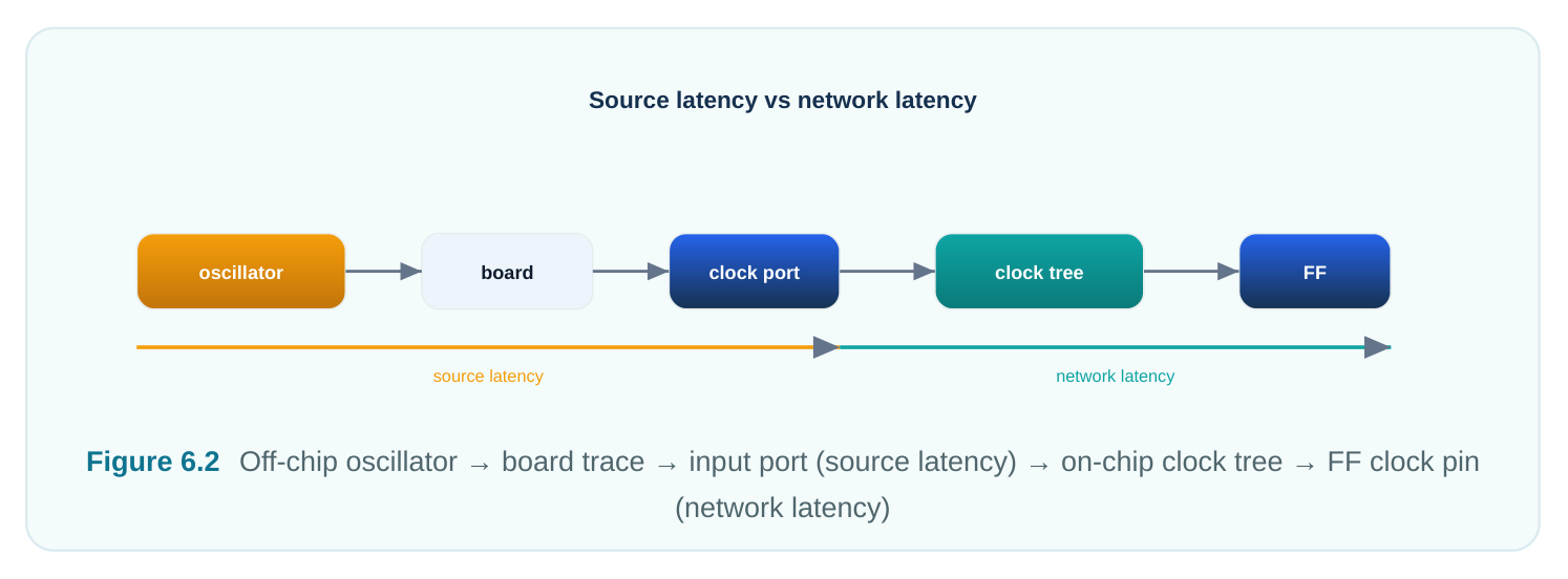
Source latency is the delay before the on-chip tree begins. Think of it as the trip to the front door. It covers the off-chip board trace, the package, and the delay up to where you declared the clock. Every register in the domain shares this delay. So on its own it makes no launch-to-capture difference. Network latency is the delay through the on-chip clock tree. This is the buffers and wires from the start point to each register's clock pin. Registers sit at different depths in the tree. So this delay differs from one endpoint to another. That difference is the physical root of skew. Common to all
Latency type Spans Source of skew?
| Source | Off-chip + up to clock definition point | Yes | No (cancels launch vs |
|---|---|---|---|
| latency | capture) | ||
| Network | Clock-definition point → each FF | No latency | Yes (differs per endpoint) clock pin |
# standard (SDC)
# 1.5 ns of off-chip / source latency on the whole CLK domain
set_clock_latency -source 1.5 [get_clocks CLK]
# 0.9 ns of network (on-chip tree) latency, used in ideal-clock mode
set_clock_latency 0.9 [get_clocks CLK]
IDEAL VS PROPAGATED CLOCK MODE
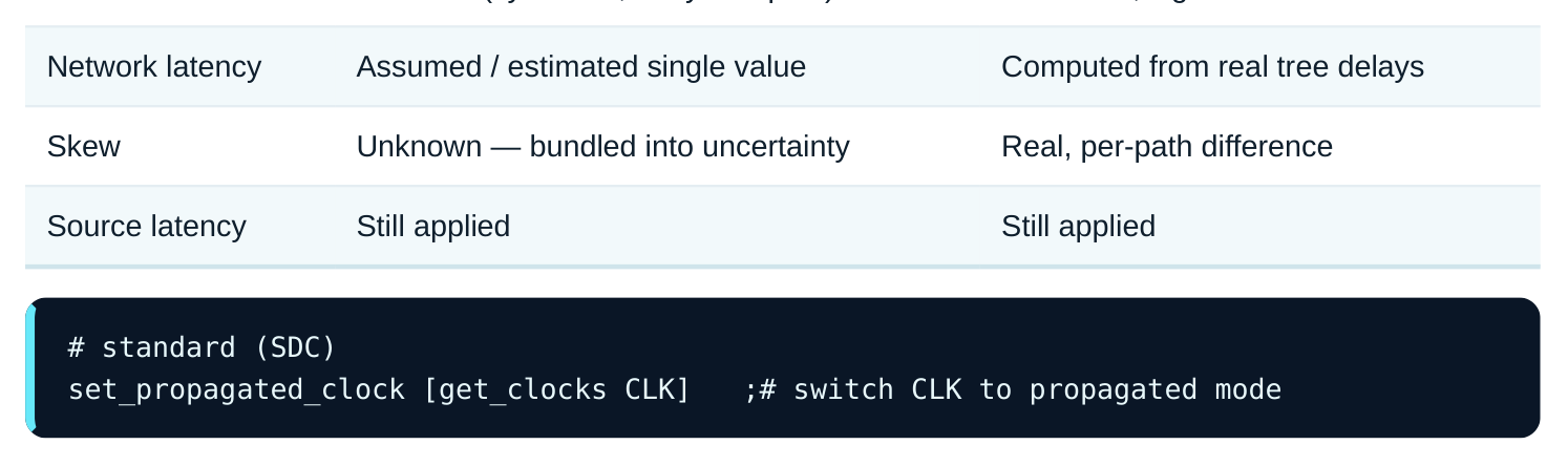
How network latency is handled depends on the mode. In ideal clock mode, the analyzer assumes a perfect tree. The clock edge reaches every register at the same time. There is no tree delay, or just one estimate you supply. This fits early in the flow. At that point no real tree exists yet. Skew is unknown. So it hides inside the uncertainty knob (§6.3). In propagated clock mode, the analyzer walks the real tree. It computes the true arrival time at each clock pin. It adds up the buffer and wire delays. Now network latency is measured, not guessed. Skew then falls out as the difference of two real arrival times. This mode is used for sign-off after clock tree synthesis (CTS, the step that builds the tree).
| Aspect | Ideal mode | Propagated mode |
|---|---|---|
| When used | Pre-CTS (synthesis, early floorplan) | Post-CTS, sign-off |
6.3 Clock Uncertainty
Before CTS you face three unknowns. You do not know the real skew. You cannot know the PLL's jitter exactly. And you want some safety margin. Modeling each one alone is hard. So STA uses one budget knob: clock uncertainty. It is a time value. The analyzer subtracts it from the timing window. It stands in for everything that makes the clock imperfect. Uncertainty bundles three things together.
| Component | What it represents | Phase of flow |
|---|---|---|
| Estimated skew | Expected spread of tree arrival times pre-CTS | Pre-CTS only |
| Jitter | Cycle-to-cycle edge variation from source/PLL | Always physical |
| Margin / guardband | Extra pessimism for modeling error, OCV, aging | Designer's choice |
The key fact is this. Uncertainty tightens both setup and hold. But it hits different edges.
- For a setup check, uncertainty is subtracted from the capture edge time. This shrinks the window the data has to arrive in. The required time moves earlier. So setup slack drops.
- For a hold check, uncertainty makes the capture edge act later than the launch. So the data must stay stable longer. Hold slack drops too. Setup and hold react to different physical effects. So most flows let you set them on their own.
# standard (SDC)# Single uncertainty applied to both setup and holdset_clock_uncertainty 0.25 [get_clocks CLK]# Split: 0.25 ns guards setup, 0.08 ns guards holdset_clock_uncertainty -setup 0.25 [get_clocks CLK]set_clock_uncertainty -hold 0.08 [get_clocks CLK]After CTS the picture changes. The real tree now exists. So real propagated skew replaces the skew part of uncertainty. You no longer need a placeholder for skew. The analyzer computes it. What is left is the part you cannot remove: jitter plus your chosen margin. A common mistake is leaving the full pre-CTS uncertainty in place after switching modes. That counts skew twice. It counts once in the real tree and once in the leftover uncertainty. The result is falsely pessimistic slack.
6.4 Skew
Clock skew is the gap in clock arrival time between the two registers on a path. It compares the launch register and the capture register.
skew = (clock arrival at capture FF) − (clock arrival at launch FF)Sign matters. Commit this convention to memory: capture minus launch. With it:
- Positive skew means the capture clock arrives later than the launch clock. The capture edge is delayed. So data gets extra time to travel. This helps setup but hurts hold.
- Negative skew means the capture clock arrives earlier. The capture edge comes sooner. So data has less time. This hurts setup but helps hold. Here is a compact way to fold skew into slack.
Setup slack = (T_period + skew) − (T_clk2q + T_logic + T_setup − T_uncertainty)
Hold slack = (T_clk2q + T_logic) − (T_hold + skew + T_uncertainty)| Skew sign | Capture edge vs launch | Setup effect | Hold effect |
|---|---|---|---|
| Positive (+) | Capture later | Helps (more time) | Hurts (data races the late edge) |
| Negative (−) | Capture earlier | Hurts (less time) | Helps |
This explains a common pattern. Hold violations often show up on short paths with positive skew. It also explains a rule for useful-skew tuning. There you delay a capture clock on purpose. This borrows time for a slow path. But you must always check the hold cost it creates. Clock skew: helps one check, hurts the other
−skew: hold easier / setup harder +skew: setup easier / hold harder
Figure 6.3 Two clock arrivals at launch and capture pins; positive skew shifting capture edge right, with arrows
showing the setup window opening and the hold window closing
6.5 Jitter
Skew is a spatial gap. It compares two points in the tree at the same cycle. Jitter is a time gap. The same edge does not arrive at the same moment every cycle. The PLL and the source oscillator make edges that wander. Power-supply noise, heat, and loop dynamics cause this. The flavor that matters most for STA is cycle-to-cycle jitter. That is the change in spacing between two edges in a row. Jitter eats setup margin. It can shorten the real clock period. Picture this. A launch edge comes a bit late. The next capture edge comes a bit early. Then the window between them is smaller than the nominal period. The analyzer must be correct in the worst case. So it assumes that squeeze on every cycle. It shrinks the setup window by the jitter amount. Jitter bites hold too. But the modeled amount is usually smaller. That is because hold uses the same edge pair within one cycle. The clock tree cannot remove jitter. It starts upstream of the chip's tree. So even a perfect zero-skew tree still has jitter. Jitter must live in the uncertainty number, or in its own budget. This is exactly why post-CTS uncertainty never reaches zero. Real skew is removed. But jitter and margin stay.
6.6 Generated-Clock Relationships and Why They Must Be Declared
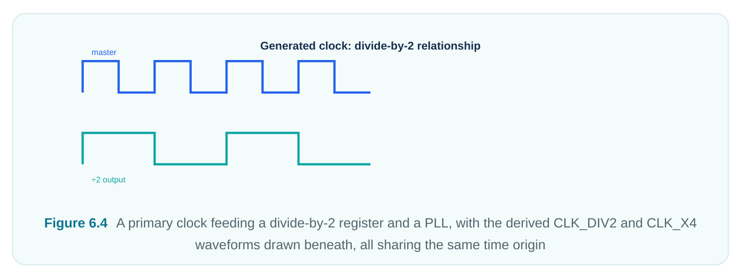
A clock can be transformed on-chip. A counter may divide it. A PLL may multiply it. A gate may simply pass it. The waveform at that node is then not the master's waveform. A generated clock declaration
fixes this. It tells the analyzer the exact period and phase between the new clock and its master. It anchors them to the master's source.
# standard (SDC)
# Divide-by-2: output toggles every master edge → period doubles
create_generated_clock -name CLK_DIV2 \
-source [get_pins div_reg/CP] -divide_by 2 \
[get_pins div_reg/Q]
# Multiply-by-4 from a PLL reference
create_generated_clock -name CLK_X4 \
-source [get_pins pll/REF] -multiply_by 4 \
[get_pins pll/CKOUT]
# Same-period derived clock through a mux/buffer (kept phase-aligned)
create_generated_clock -name CLK_GATED \
-source [get_pins gate/A] -divide_by 1 \
[get_pins gate/Z]
Why is the declaration required? There are two reasons. First, correct timing math. Say a divide-by-2 register feeds logic. Suppose the analyzer still thinks the downstream clock has the master's period. Then it checks setup against the wrong period. That period is too tight. The slack it reports is nonsense. Declaring the generated clock gives the true period and the right edge alignment. Second, correct links between domains. Generated clocks from the same master share one origin. So the analyzer can pair launch and capture edges between a master domain and a derived one. An example is a path from a full-rate domain into a half-rate domain. Without the declaration the tool may treat them as unrelated. It may then mishandle the crossing. It could miss a real violation or report a false one. One subtle point matters. A generated clock's latency is referenced through its master's source. So source latency on the master flows into the generated clock by itself. You can still add network latency local to the generated node. Getting this order right keeps multi-rate and PLL designs analyzable.
6.7 Reading a Clock Report
Below is an illustrative report fragment. It shows how the clock model appears in a path. Watch how source latency, network latency, and uncertainty each show up on their own. Note that the launch and capture columns differ only by network latency (skew) and the period.
# illustrative — generic, not tool-specific
Clock: CLK   Period: 10.000   Mode: propagated
Launch path (data launched at FF_A/CK):
clock source                    0.000
+ source latency                1.500
+ network latency (to FF_A)     0.700   -> launch edge = 2.200
Capture path (data captured at FF_B/CK):
clock edge (period)            10.000
+ source latency                1.500
+ network latency (to FF_B)     0.810   -> capture edge = 12.310
- setup uncertainty (jitter+margin)  0.120  -> required = 12.190
Skew (capture 0.810 - launch 0.700) = +0.110  (helps setup)
Two checks an interviewer loves. First, confirm source latency appears the same on both sides. It cancels for skew. Second, confirm uncertainty is subtracted on the capture side for a setup check.
Interview Q&A
unchanged. What's the problem? You count skew twice. Pre-CTS, uncertainty bundles a skew estimate plus jitter plus margin. Once propagated, the analyzer computes the real skew from the tree. So the estimate inside uncertainty is now redundant. Leaving it in piles pessimism on top of physical skew. That gives artificially negative slack. The fix is simple. Drop uncertainty to just jitter plus margin after switching to propagated clocks.
helps setup but hurts hold. Positive skew means the capture edge arrives later than the launch edge. For setup, a later capture edge widens the window the data can arrive in. So there is more time and slack improves. For hold, that same later capture edge gives the new data launched this cycle more chance to reach the capture flop before it samples. So the stored value can be corrupted. The hold check gets harder and slack worsens.
delay before the tree begins. It is common to every register. It appears the same on both launch and capture paths. So it cancels in the difference. Network latency is the per-endpoint delay through the tree. It differs between any two registers by their depth and routing. That difference is skew.
zero? Because jitter and margin remain. Jitter starts in the PLL or source upstream of the tree. So a balanced tree cannot remove it. Consecutive edges still vary in spacing. That compresses the real period and eats setup margin. On top of that, engineers keep a guardband. It covers modeling error, on-chip variation, and aging. So post-CTS uncertainty settles at jitter plus margin, not zero.
Key Takeaways
- A clock is defined by period, waveform (edges/duty cycle), and source. Primary clocks are roots. Generated clocks (divided, multiplied, gated) are tied to a master by math and must be declared for correct period, phase, and cross-domain analysis.
- Latency splits into source latency (off-chip, common to all sinks, cancels for skew) and network latency (per-endpoint tree delay, the physical root of skew).
- Ideal mode assumes a perfect tree pre-CTS. Propagated mode computes real arrival times post- CTS and exposes real skew.
- Clock uncertainty is one pre-CTS knob bundling estimated skew + jitter + margin. It tightens both setup and hold. After CTS the skew part is replaced by real propagated skew, leaving jitter + margin.
- Skew (capture − launch): positive helps setup and hurts hold; negative hurts setup and helps hold. Jitter is cycle-to-cycle edge variation from the source/PLL. It compresses the real period and eats setup margin. It never fully disappears, no matter how balanced the tree.
Comments
Leave a Reply