 ChipBuddy
← Home
ChipBuddy
← Home
Clock Latency, Uncertainty & Jitter
Clock Latency, Uncertainty & Jitter
A clock signal does not appear everywhere at the same instant. It starts somewhere off-chip or at a pin, travels through wires and buffers, and arrives at each flip-flop a little later. A flip-flop is a storage element that captures data on a clock edge. The time the clock takes to reach a flip-flop is called clock latency. The timing tool needs to know this latency to compute when each edge truly arrives. Real clocks are also not perfectly steady. The exact edge time wobbles a bit from cycle to cycle. We capture all of this wobble and modeling slop with a single number called clock uncertainty. This chapter explains how the SDC constraint format describes both latency and uncertainty, and how they change the setup and hold checks. A setup check asks whether data arrives early enough before the capturing edge. A hold check asks whether data stays stable long enough after the edge. Latency and uncertainty both nudge these two checks, and they nudge them in opposite directions. Before going further it helps to see why latency and uncertainty are separate ideas. Latency is about average position: where, on average, the clock edge lands at a flip-flop. Uncertainty is about spread: how far the real edge might stray from that average on any given cycle. A path can have large latency but tiny uncertainty, or small latency but large uncertainty. The tool needs both. Latency shifts the whole check in time; uncertainty shrinks the safe window around it. Keeping the two ideas distinct prevents a lot of confusion when reading timing reports.
Source Latency vs Network Latency
Clock latency splits into two parts. Source latency is the delay from the true clock origin (a board oscillator or an upstream chip) to the clock port of our chip. Network latency is the delay from that port through the on-chip clock distribution to each flip-flop. The on-chip distribution is the clock tree, a balanced web of buffers that fans the clock out to thousands of flip-flops. We separate the two because they behave differently. Source latency is usually the same for every flip-flop on one clock, since it happens before the clock enters the chip. Network latency differs from flip-flop to flip-flop, because some are near the clock root and some are far. The difference in network latency between two flip-flops is clock skew. The set_clock_latency command sets both kinds. With no special option it sets source-plusnetwork as a combined value. With the -source option it sets only the source part. A realistic source latency might be 1.35 ns; a realistic network latency before the tree is built might be 0.80 ns.
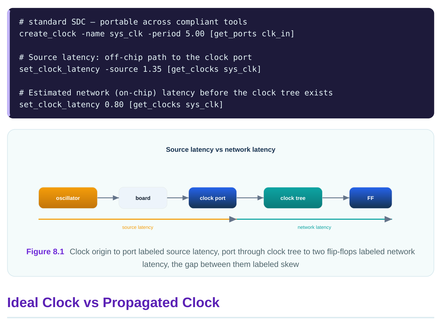
Early in the flow, the clock tree does not exist yet. The tool treats the clock as ideal, meaning the clock reaches every flip-flop at the same modeled time. With an ideal clock, network latency is whatever number you typed with set_clock_latency , and skew is zero unless you add it through uncertainty.
After the clock tree is built, the tool switches to a propagated clock. Now it computes real arrival times by adding up the actual buffer and wire delays in the tree. Network latency becomes a measured value, and skew falls out of the real structure. You enable this with set_propagated_clock . The two stages are usually called pre-CTS and post-CTS, where CTS means clock tree synthesis, the step that builds the balanced tree. Pre-CTS the clock is ideal and you model skew with uncertainty. Post-CTS the clock is propagated and real skew is already counted, so you can shrink the uncertainty number.
| Stage | Clock mode | Network latency source | Skew handling |
|---|---|---|---|
| Pre-CTS | Ideal | Typed estimate (e.g. 0.80 ns) | Bundled into uncertainty |
| Post-CTS | Propagated | Computed from real tree | Real skew counted directly |
| Sign-off | Propagated | Computed, with parasitics | Real skew plus small margin |
Clock Uncertainty: One Number for Many Effects
set_clock_uncertainty adds a guard band to clock-based checks. It is a single number that bundlesseveral real effects so you do not have to model each one separately. The main ingredients are clock skew, clock jitter, and design margin. Jitter is the cycle-to-cycle variation in the clock edge time, caused by the oscillator and power supply noise. Margin is extra pessimism the team adds on purpose to stay safe. Pre-CTS, skew is also folded in because the tool has no real tree to measure. A typical pre-CTS setup uncertainty might be 0.30 ns. A typical hold uncertainty might be 0.08 ns. You can set different values for setup and hold using the -setup and -hold options, which matters because the two checks want different margins.
# standard SDC — portable across compliant tools
# Pre-CTS: larger setup uncertainty bundles skew + jitter + margin
set_clock_uncertainty -setup 0.30 [get_clocks sys_clk]
set_clock_uncertainty -hold 0.08 [get_clocks sys_clk]| Effect | In setup uncertainty? | In hold uncertainty? | Typical share |
|---|---|---|---|
| Clock skew (pre-CTS) | Yes | Yes | 0.10–0.15 ns |
| Jitter | Yes | Small | 0.05–0.10 ns |
| Design margin | Yes | Yes | 0.05–0.10 ns |
How Uncertainty Tightens Setup and Hold
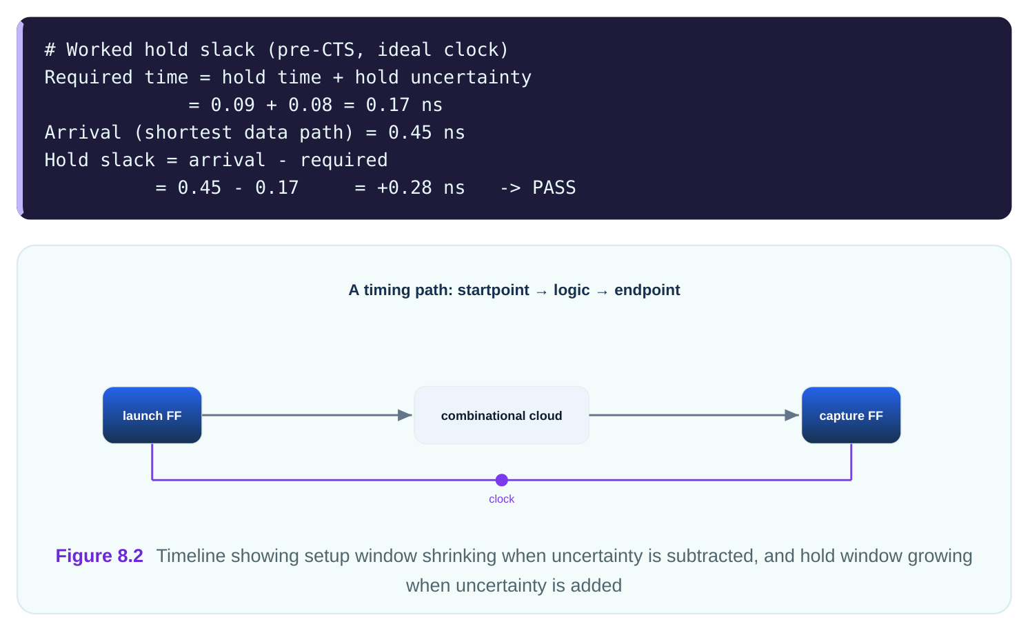
Uncertainty makes both checks harder, but through opposite math. For setup, the tool subtracts the uncertainty from the time available, so the data must arrive earlier. For hold, the tool adds the uncertainty to the required hold time, so the data must stay stable longer. In both cases you lose margin. The amount of margin you have is called slack. Positive slack means the path passes; negative slack means it fails. Uncertainty is a direct tax on slack. Here is a worked setup example. Suppose the clock period is 5.00 ns. The data path from launch flipflop to capture flip-flop takes 4.10 ns. The capture flip-flop needs a setup time of 0.12 ns. Setup uncertainty is 0.30 ns.
# Worked setup slack (pre-CTS, ideal clock)
Capture edge (period)        = 5.00 ns
Minus setup time             = -0.12 ns
Minus setup uncertainty      = -0.30 ns
Required time                =  4.58 ns
Arrival (data path delay)    =  4.10 ns
Setup slack = 4.58 - 4.10    = +0.48 ns   -> PASS
Now a hold example on the same path. Hold checks use the same launch edge. The shortest data path is 0.45 ns. The capture flip-flop needs a hold time of 0.09 ns. Hold uncertainty is 0.08 ns.
Pre-CTS to Post-CTS: Shrinking the Number
The whole point of building a real clock tree is to replace guesses with measurements. Pre-CTS you do not know the skew, so you pad uncertainty heavily. Post-CTS the tool knows the real skew from the propagated clock, so you can drop the skew portion out of uncertainty and keep only jitter and margin. A common pattern: pre-CTS setup uncertainty 0.30 ns, post-CTS setup uncertainty 0.12 ns. The 0.18 ns difference is roughly the skew you no longer need to guess at. Forgetting to lower the number postCTS leaves you with double pessimism, which makes paths look worse than they are and wastes area on over-fixing. There is a symmetric trap on the hold side. Real skew can help or hurt hold depending on direction. If the capture clock arrives later than the launch clock, that skew eats into the hold margin. Pre-CTS you padded hold uncertainty to cover this unknown. Post-CTS the propagated tree shows the true skew, so you set hold uncertainty to just jitter and margin, perhaps 0.06 ns. Getting this right keeps the tool from inserting unnecessary hold-fixing delay cells, which cost both area and dynamic power.
# standard SDC — portable across compliant tools
# Post-CTS: clock now propagated, real skew counted, uncertainty shrinks
set_propagated_clock [get_clocks sys_clk]
set_clock_uncertainty -setup 0.12 [get_clocks sys_clk]
set_clock_uncertainty -hold  0.06 [get_clocks sys_clk]
To see the breakdown a tool gives, a report command helps. The exact flags differ by tool.
delay from the true clock origin to the chip's clock port, for example 1.35 ns off-chip. Network latency is the delay from that port through the on-chip clock tree to each flip-flop, for example 0.80 ns. Source latency is shared by all flip-flops on the clock; network latency varies per flip-flop, and that variation is skew.
the SDC level the tool just needs a single guard band to subtract or add during checks. Bundling keeps constraints simple. Pre-CTS a setup uncertainty of 0.30 ns might be 0.12 ns skew, 0.10 ns jitter, and 0.08 ns margin. The tool does not care about the split; it only applies the total.
time, so data must arrive earlier. For hold it is added to the required time, so data must stay stable
longer. Both reduce slack. That is why teams set them separately, often 0.30 ns for setup and 0.08 ns for hold.
network latency is a typed estimate, so skew is unknown and folded into uncertainty. Post-CTS the clock is propagated, real skew is measured from the tree, so you remove the skew portion and shrink uncertainty, say from 0.30 ns to 0.12 ns.
What is the setup slack? Required time is 5.00 - 0.12 - 0.30 = 4.58 ns. Arrival is 4.40 ns. Setup slack is 4.58 - 4.40 = +0.18 ns. It passes, but with little margin.
the real propagated tree and once in the still-large uncertainty number. Paths look more negative than reality. The tool over-fixes, adding buffers and area you did not need, and may report false setup violations.
Key Takeaways
- Clock latency splits into source (origin to port) and network (port to flip-flop through the tree); their difference is skew.
- An ideal clock uses typed latency with zero real skew; a propagated clock computes real arrival times after CTS.
- set_clock_uncertainty bundles skew, jitter, and margin into one guard band, often set separately for setup and hold.
- Uncertainty is subtracted for setup and added for hold, taxing slack in both directions.
- Move from a large pre-CTS uncertainty to a smaller post-CTS value once real skew is measured, or you double-count pessimism.
Comments
Leave a Reply