 ChipBuddy
← Home
ChipBuddy
← Home
Clock Latency — Source vs Network
Clock Latency — Source vs Network (Deep)
A clock edge does not appear everywhere at once. It starts at a source and travels through wires and buffers to reach each flip-flop. That travel takes time. The total travel time is the clock latency, also called insertion delay. This chapter goes deep on set_clock_latency . It separates source latency from network latency. It contrasts the ideal-clock and propagated-clock views. It shows how to model latency before the clock tree is built. And it explains how latency shifts the launch and capture edges of a timing check.
Two Parts of Clock Latency
Clock latency splits into two parts. The split matters because the two parts behave differently in analysis. Source latency is the delay from the clock's true origin to the clock's definition point on the chip. The origin might be an off-chip oscillator or an on-chip generator. The definition point is the port or pin where you write create_clock . Source latency models everything before the chip's clock entry. Network latency is the delay from the definition point to each flip-flop's clock pin, inside the chip. This is the on-chip clock tree. The clock tree is the web of buffers and wires that fans the clock out to thousands of flops.
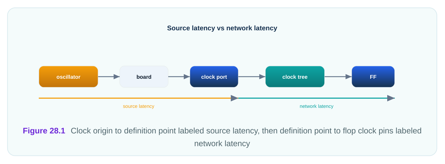
The total insertion delay at any flop is source latency plus network latency. If source latency is 1.73 ns and network latency to a given flop is 0.94 ns, that flop sees its clock edge 2.67 ns after the true origin.
| Latency part | From | To | Models |
|---|---|---|---|
| Source | Clock origin | Definition point | Off-chip path, board, generator |
| Network | Definition point | Flop clock pin | On-chip clock tree |
| Insertion delay | Origin | Flop clock pin | Source + network total |
Ideal vs Propagated Clocks
There are two ways the tool can treat the clock tree. The choice depends on where you are in the flow. An ideal clock has no real network delay. The tool pretends the clock reaches every flop at the same instant. This is used early, before the clock tree exists. You have netlist and clocks but no real tree yet. The ideal view lets you check logic timing without a tree. A propagated clock uses the real delays through the actual clock tree. Every buffer and wire counts. This is used after the tree is built, when the real delays are known. The propagated view is the accurate one.
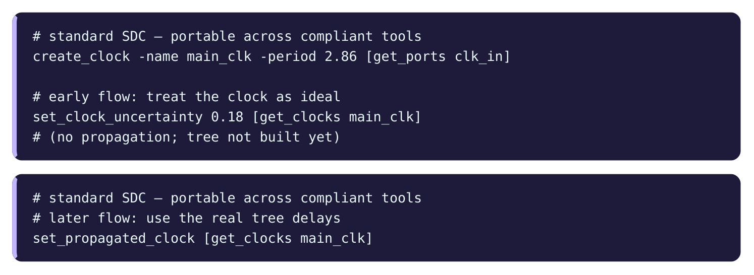
When a clock is ideal, you still want to model the tree's effect roughly. That is where source latency, and modeled network latency, come in. You stand in for the missing tree with hand-set numbers.
| View | Network delay | When used | Accuracy |
|---|---|---|---|
| Ideal | Zero (or modeled) | Before clock tree built | Rough |
| Propagated | Real tree delays | After clock tree built | Accurate |
Modeling Latency Before the Tree Exists
Before the clock tree is built, the tool does not know the network delay. But you can estimate it. You tell the tool an expected insertion delay so early timing checks are realistic.
set_clock_latency -source sets the source part. set_clock_latency without -source sets thenetwork part. On an ideal clock, the network latency you set stands in for the not-yet-built tree.
# standard SDC — portable across compliant tools
create_clock -name sys_clk -period 3.42 [get_ports clk_in]
# source latency: origin to definition point
set_clock_latency -source 1.73 [get_clocks sys_clk]
# modeled network latency: stand-in for the future tree
set_clock_latency 0.94 [get_clocks sys_clk]
Why bother? Because launch and capture flops may sit at different depths in the future tree. If you model a network latency, the tool can see roughly how the tree will shift edges. This makes pre-tree timing closer to the truth. When the real tree is built, you switch to set_propagated_clock and the modeled network latency is replaced by real delays. The source latency usually stays, because the off-chip path does not change. There is a subtle benefit. By modeling source latency separately, you keep the off-chip part fixed across the whole flow. Only the on-chip part changes when you go from ideal to propagated. This separation keeps your constraints stable.
How Latency Shifts Launch and Capture
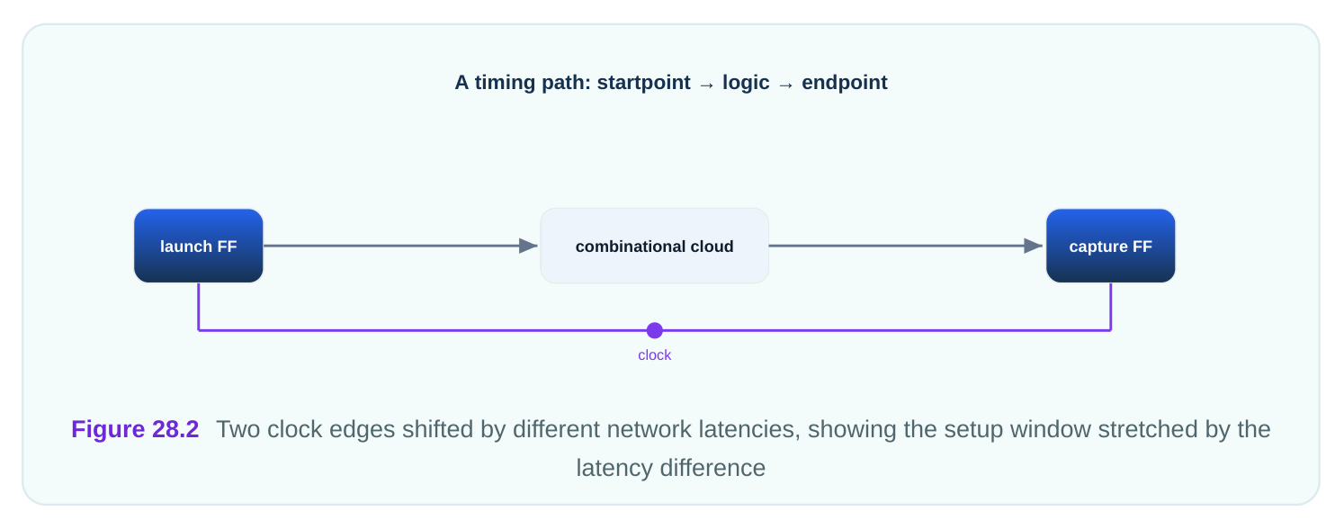
A timing check compares two edges. The launch edge is when the source flop sends data. The capture edge is when the destination flop catches it. Both edges are shifted by the latency to their respective clock pins. Here is the key idea. The setup check measures from the launch edge plus launch latency, to the capture edge plus capture latency. If the two flops have different latencies, the difference shifts the whole check.
Let us work an example. Same clock, two flops, different network latencies.
# Worked illustrative example — latency shifting a setup check
Clock period                    = 3.42 ns
Source latency (both flops)     = 1.73 ns
Launch flop network latency     = 0.94 ns
Capture flop network latency    = 1.11 ns
Launch edge arrives at source flop  = 1.73 + 0.94      = 2.67 ns
Capture edge arrives at dest flop   = 3.42 + 1.73 + 1.11 = 6.26 ns
Time available launch to capture    = 6.26 - 2.67      = 3.59 ns
Notice the available time is 3.59 ns, not the bare 3.42 ns period. The capture flop's larger network latency, 1.11 ns versus 0.94 ns, pushed its edge later by 0.17 ns. That extra 0.17 ns helps setup. This is the effect of latency skew between launch and capture. Now flip it. If the capture flop had the smaller latency, its edge would come earlier, and setup would lose time. The direction of the latency difference decides whether setup gains or loses.
| Case | Capture latency vs launch | Effect on setup |
|---|---|---|
| Capture later | Larger | More time, setup helped |
| Capture earlier | Smaller | Less time, setup hurt |
| Equal | Same | No shift, period unchanged |
For hold, the logic reverses. Hold compares edges in the same cycle, so a later capture edge hurts hold. This is why latency skew is a double-edged sword: what helps setup can hurt hold.
Insertion Delay and Why It Matters
Insertion delay is the total clock latency at a flop, source plus network. It is the single number that says how late the clock arrives at that flop.
Insertion delay matters most for crossings and for the relationship between clocks. Two clocks with very different insertion delays will have their edges offset. That offset enters every check between them. Consider input and output delays at chip boundaries. The source latency of your clock affects how the outside world's data lines up with your internal clock. If your source latency is 1.73 ns, your internal capture edge is 1.73 ns later than the clock at the port. Your input delay numbers must account for this, or the boundary timing is wrong. A common pitfall is changing latency modeling between flow stages without updating boundary delays. If early timing uses a 0.94 ns modeled network latency but the real tree comes in at 1.31 ns, the boundary timing shifts by 0.37 ns. If you do not re-check the boundaries, a passing path may turn failing.
| Insertion delay use | Why it matters |
|---|---|
| Cross-clock checks | Edge offset enters every check |
| Boundary delays | Internal edge shifts vs port clock |
| Setup/hold tradeoff | Latency skew helps one, hurts other |
| Flow consistency | Modeled vs real must be reconciled |
To inspect latency, you ask the tool to report it per clock and per flop.
# illustrative — names vary by tool
report_clock -latency [get_clocks sys_clk]
report_timing -from [get_pins launch_reg/CK] -to [get_pins cap_reg/D]
The reports show the source and network parts so you can confirm the numbers match your intent and the real tree.
Interview Q&A
delay from the clock's true origin to its definition point on the chip, modeling the off-chip path and any generator. Network latency is the delay from the definition point to each flop's clock pin, modeling the on-chip clock tree. Their sum is the insertion delay. For example, 1.73 ns source plus 0.94 ns network gives 2.67 ns at the flop.
before the clock tree is built, when the network delay is unknown. The tool pretends the clock reaches all flops at once, though you can model the network latency by hand. You switch to a propagated clock after the tree is built, using set_propagated_clock , so the real buffer and wire delays are used.
flops will sit at different tree depths, and modeling latency lets early timing reflect that.
set_clock_latency -source sets the off-chip part and set_clock_latency sets the modeled on-chip part. When the real tree arrives, propagation replaces the modeled network part while the source part usually stays fixed.
latency is larger, its edge comes later, giving the path more time, which helps setup. If the capture latency is smaller, the edge comes earlier and setup loses time. With a 0.94 ns launch and 1.11 ns capture network latency, the capture edge is 0.17 ns later, adding 0.17 ns to the setup window.
compares edges across cycles, so a later capture edge gives more time. Hold compares edges in the same cycle, so a later capture edge gives less margin. A 0.17 ns latency difference that helps setup by 0.17 ns can hurt hold by a similar amount.
internal clock edge relative to the clock at the port. With a 1.73 ns source latency, the internal capture edge is 1.73 ns later than the port clock. Your input and output delay numbers must account for that shift, or the boundary timing is wrong. Changing the latency model later without re-checking boundaries can flip a passing path to failing.
Key Takeaways
- Source latency covers the origin-to-definition path and network latency covers the on-chip clock tree; their sum is the insertion delay at each flop.
- Ideal clocks are for the pre-tree flow with zero or modeled network delay; propagated clocks use real tree delays after the tree is built.
- Model source and network latency early so pre-tree timing reflects how the future tree will shift edges.
- Latency skew shifts the launch and capture edges: a later capture edge helps setup but hurts hold, so it cuts both ways.
- Source latency shifts internal edges versus the port clock, so boundary delays must track any change in the latency model.
Comments
Leave a Reply